Table of Contents
Path Analysis
Introduction
Regressions vs. Path Analysis (or SEM)
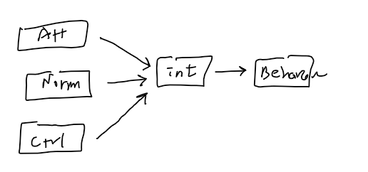
- Intention = a1 + b1(Attitude) + b2(Norms) + b3(Control)
- Behavior = a2 + b4(Intention)
- When in a combined situation, we use
- Path Analysis or SEM
Model Identification
- Terms
- The number of unique (non-redundent) source of information
- $p(p+1)/2$
- The number of parameters (paths) specified in model
- Just-identified (df = 0)
- Model can be estimated, but cannot be assessed
- Over-identified (df > 0)
- Model can be estimated and assessed
- Under-identified (df < 0)
- Model cannot be either estimated or assessed
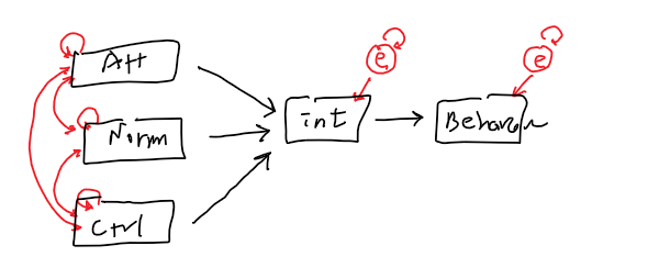
- Exogenous and
- Endogenous Variables
- Covariance
- Variance
- Path coefficient
- Residual error
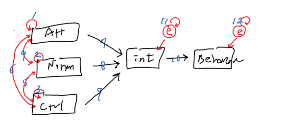
out of possible 15 relationships
15 - 12 =3 (df)
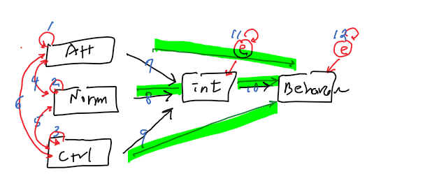
- Model fit
- Chi-square Test: p-value less than p-critical value (.05 for example) indicates that model does not fit well enough. p-value more than critical value means the model fits the data relatively well. The test is sensitive to the sample size and normality of the data.
- CFI (Comparative Fit Index): greater than .90 indicates good fit to the data. It is less sensitive to the sample size and normality of the data than chi-square test.
- TLI (Tucker-Lewis Index): greater than .95 (sometimes .90) indicates good fit. It is less sensitive to the sample size.
- RMSEA (Root Mean Square Error of Approximation): equal to or less than .08 (sometimes .10 is used) indicates good fit to the data.
- SRMR (Standard Root Mean square Residual): less than or equal to .08 indicates good fit to the data.
| $\chi^2$ | $\text{CFI}$ | $\text{TLI}$ | $\text{RMSEA}$ | $\text{SRMR}$ |
| $p \ge .05$ | $p \ge .90$ | $p \ge .95$ | $p \le .08$ | $p \le .08$ |
Then what is SEM (Structural Equation Modeling)
- Relationships within and among variables and constructs
E.g. in R
######################################################
## data file: PlannedBehavior.csv
######################################################
######################################################
install.packages("readr")
library(readr)
df <- read.csv("http://commres.net/wiki/_media/r/plannedbehavior.csv")
head(df)
str(df)

# path analysis in R using lavaan package
# install.packages("lavaan")
library(lavaan)

# Model speficiation
specmod <- "
    intention ~ attitude + norms + control
"
# Estimate model
fitmod <- sem(specmod, data=df)

# summarize the result
summary(fitmod, fit.measures=TRUE, rsquare=TRUE)
specmod2
# Model speficiation 2
specmod2 <- "
    intention ~ attitude + norms + control
    attitude ~~ norms + control
    norms ~~ control
"
fitmod2 <- sem(specmod2, data=df)

# summarize the result
summary(fitmod2, fit.measures=TRUE, rsquare=TRUE)
specmod3: lm
fitmod3 <- lm(intention~attitude+norms+control, data=df)
summary(fitmod3)
specmod4
# pbt model
specmod4 <- "
    # Directional relations (path)
    intention ~ attitude + norms + control
    behavior ~ intention
    # Covariances
    attitude ~~ norms + control
    norms ~~ control
"
fitmod4 <- sem(specmod4, data=df)
summary(fitmod4, fit.measures=TRUE, rsquare=TRUE)
# my own
# pbt model
specmod5 <- '
    # Directional relations (path)
    intention ~ a*attitude + b*norms + c*control
    behavior ~ d*intention
    # Covariances
    attitude ~~ norms + control
    norms ~~ control
    ad := a*d
    bd := b*d
    cd := c*d
'
fitmod5 <- sem(specmod5, data=df)
summary(fitmod5, fit.measures=TRUE, rsquare=TRUE)
Output
> df <- read.csv("http://commres.net/wiki/_media/r/plannedbehavior.csv")
> head(df)
  attitude norms control intention behavior
1     2.31  2.31    2.03      2.50     2.62
2     4.66  4.01    3.63      3.99     3.64
3     3.85  3.56    4.20      4.35     3.83
4     4.24  2.25    2.84      1.51     2.25
5     2.91  3.31    2.40      1.45     2.00
6     2.99  2.51    2.95      2.59     2.20
> str(df)
'data.frame':	199 obs. of  5 variables:
 $ attitude : num  2.31 4.66 3.85 4.24 2.91 2.99 3.96 3.01 4.77 3.67 ...
 $ norms    : num  2.31 4.01 3.56 2.25 3.31 2.51 4.65 2.98 3.09 3.63 ...
 $ control  : num  2.03 3.63 4.2 2.84 2.4 2.95 3.77 1.9 3.83 5 ...
 $ intention: num  2.5 3.99 4.35 1.51 1.45 2.59 4.08 2.58 4.87 3.09 ...
 $ behavior : num  2.62 3.64 3.83 2.25 2 2.2 4.41 4.15 4.35 3.95 ...
>
> # path analysis in R using lavaan package
> # install.packages("lavaan")
> library(lavaan)
This is lavaan 0.6-9
lavaan is FREE software! Please report any bugs.
Warning message:
패키지 ‘lavaan’는 R 버전 4.1.2에서 작성되었습니다
>
> # Model speficiation
> specmod <- "
+     intention ~ attitude + norms + control
+ "
> # Estimate model
> fitmod <- sem(specmod, data=df)
>
> # summarize the result
> summary(fitmod, fit.measures=TRUE, rsquare=TRUE)
lavaan 0.6-9 ended normally after 11 iterations

  Estimator                                         ML
  Optimization method                           NLMINB
  Number of model parameters                         4

  Number of observations                           199

Model Test User Model:

  Test statistic                                 0.000
  Degrees of freedom                                 0

Model Test Baseline Model:

  Test statistic                                91.633
  Degrees of freedom                                 3
  P-value                                        0.000

User Model versus Baseline Model:

  Comparative Fit Index (CFI)                    1.000
  Tucker-Lewis Index (TLI)                       1.000

Loglikelihood and Information Criteria:

  Loglikelihood user model (H0)               -219.244
  Loglikelihood unrestricted model (H1)       -219.244

  Akaike (AIC)                                 446.489
  Bayesian (BIC)                               459.662
  Sample-size adjusted Bayesian (BIC)          446.990

Root Mean Square Error of Approximation:

  RMSEA                                          0.000
  90 Percent confidence interval - lower         0.000
  90 Percent confidence interval - upper         0.000
  P-value RMSEA <= 0.05                             NA

Standardized Root Mean Square Residual:

  SRMR                                           0.000

Parameter Estimates:

  Standard errors                             Standard
  Information                                 Expected
  Information saturated (h1) model          Structured

Regressions:
                   Estimate  Std.Err  z-value  P(>|z|)
  intention ~
    attitude          0.352    0.058    6.068    0.000
    norms             0.153    0.059    2.577    0.010
    control           0.275    0.058    4.740    0.000

Variances:
                   Estimate  Std.Err  z-value  P(>|z|)
   .intention         0.530    0.053    9.975    0.000

R-Square:
                   Estimate
    intention         0.369
specmod2:
> # Model speficiation 2
> specmod2 <- "
+     intention ~ attitude + norms + control
+     attitude ~~ norms + control
+     norms ~~ control
+ "
> fitmod2 <- sem(specmod2, data=df)
>
> # summarize the result
> summary(fitmod2, fit.measures=TRUE, rsquare=TRUE)
lavaan 0.6-9 ended normally after 17 iterations

  Estimator                                         ML
  Optimization method                           NLMINB
  Number of model parameters                        10

  Number of observations                           199

Model Test User Model:

  Test statistic                                 0.000
  Degrees of freedom                                 0

Model Test Baseline Model:

  Test statistic                               136.306
  Degrees of freedom                                 6
  P-value                                        0.000

User Model versus Baseline Model:

  Comparative Fit Index (CFI)                    1.000
  Tucker-Lewis Index (TLI)                       1.000

Loglikelihood and Information Criteria:

  Loglikelihood user model (H0)              -1011.828
  Loglikelihood unrestricted model (H1)      -1011.828

  Akaike (AIC)                                2043.656
  Bayesian (BIC)                              2076.589
  Sample-size adjusted Bayesian (BIC)         2044.908

Root Mean Square Error of Approximation:

  RMSEA                                          0.000
  90 Percent confidence interval - lower         0.000
  90 Percent confidence interval - upper         0.000
  P-value RMSEA <= 0.05                             NA

Standardized Root Mean Square Residual:

  SRMR                                           0.000

Parameter Estimates:

  Standard errors                             Standard
  Information                                 Expected
  Information saturated (h1) model          Structured

Regressions:
                   Estimate  Std.Err  z-value  P(>|z|)
  intention ~
    attitude          0.352    0.058    6.068    0.000
    norms             0.153    0.059    2.577    0.010
    control           0.275    0.058    4.740    0.000

Covariances:
                   Estimate  Std.Err  z-value  P(>|z|)
  attitude ~~
    norms             0.200    0.064    3.128    0.002
    control           0.334    0.070    4.748    0.000
  norms ~~
    control           0.220    0.065    3.411    0.001

Variances:
                   Estimate  Std.Err  z-value  P(>|z|)
   .intention         0.530    0.053    9.975    0.000
    attitude          0.928    0.093    9.975    0.000
    norms             0.830    0.083    9.975    0.000
    control           0.939    0.094    9.975    0.000

R-Square:
                   Estimate
    intention         0.369
specmod3: lm
> fitmod3 <- lm(intention~attitude+norms+control, data=df)
> summary(fitmod3)

Call:
lm(formula = intention ~ attitude + norms + control, data = df)

Residuals:
     Min       1Q   Median       3Q      Max
-1.80282 -0.52734 -0.06018  0.51228  1.85202

Coefficients:
            Estimate Std. Error t value Pr(>|t|)
(Intercept)  0.58579    0.23963   2.445   0.0154 *
attitude     0.35232    0.05866   6.006 9.13e-09 ***
norms        0.15250    0.05979   2.550   0.0115 *
control      0.27502    0.05862   4.692 5.09e-06 ***
---
Signif. codes:  0 ‘***’ 0.001 ‘**’ 0.01 ‘*’ 0.05 ‘.’ 0.1 ‘ ’ 1

Residual standard error: 0.7356 on 195 degrees of freedom
Multiple R-squared:  0.369,	Adjusted R-squared:  0.3593
F-statistic: 38.01 on 3 and 195 DF,  p-value: < 2.2e-16
specmod4
>
> # pbt model
> specmod4 <- "
+     # Directional relations (path)
+     intention ~ attitude + norms + control
+     behavior ~ intention
+     # Covariances
+     attitude ~~ norms + control
+     norms ~~ control
+ "
> fitmod4 <- sem(specmod4, data=df)
> summary(fitmod4, fit.measures=TRUE, rsquare=TRUE)
lavaan 0.6-9 ended normally after 17 iterations

  Estimator                                         ML
  Optimization method                           NLMINB
  Number of model parameters                        12

  Number of observations                           199

# chi-square test
# p-value is over .05 indicating . . . .
Model Test User Model:

  Test statistic                                 2.023
  Degrees of freedom                                 3
  P-value (Chi-square)                           0.568

Model Test Baseline Model:

  Test statistic                               182.295
  Degrees of freedom                                10
  P-value                                        0.000

# CFI >_ .90
# TLI >_ .95
# The two indicate that the model fits to the data well

User Model versus Baseline Model:

  Comparative Fit Index (CFI)                    1.000
  Tucker-Lewis Index (TLI)                       1.019

Loglikelihood and Information Criteria:

  Loglikelihood user model (H0)              -1258.517
  Loglikelihood unrestricted model (H1)      -1257.506

  Akaike (AIC)                                2541.035
  Bayesian (BIC)                              2580.555
  Sample-size adjusted Bayesian (BIC)         2542.538

# RMSEA <_ .08
#
Root Mean Square Error of Approximation:

  RMSEA                                          0.000
  90 Percent confidence interval - lower         0.000
  90 Percent confidence interval - upper         0.103
  P-value RMSEA <= 0.05                          0.735

# SRMR <_ .08 meets the standard
#
Standardized Root Mean Square Residual:

  SRMR                                           0.019

Parameter Estimates:

  Standard errors                             Standard
  Information                                 Expected
  Information saturated (h1) model          Structured

Regressions:
                   Estimate  Std.Err  z-value  P(>|z|)
  intention ~
    attitude          0.352    0.058    6.068    0.000
    norms             0.153    0.059    2.577    0.010
    control           0.275    0.058    4.740    0.000
  behavior ~
    intention         0.453    0.065    7.014    0.000

Covariances:
                   Estimate  Std.Err  z-value  P(>|z|)
  attitude ~~
    norms             0.200    0.064    3.128    0.002
    control           0.334    0.070    4.748    0.000
  norms ~~
    control           0.220    0.065    3.411    0.001

Variances:
                   Estimate  Std.Err  z-value  P(>|z|)
   .intention         0.530    0.053    9.975    0.000
   .behavior          0.699    0.070    9.975    0.000
    attitude          0.928    0.093    9.975    0.000
    norms             0.830    0.083    9.975    0.000
    control           0.939    0.094    9.975    0.000

R-Square:
                   Estimate
    intention         0.369
    behavior          0.198
specmod5
> specmod5 <- "
+     # Directional relations (path)
+     intention ~ attitude + norms + control
+     behavior ~ intention + norms
+     # Covariances
+     attitude ~~ norms + control
+     norms ~~ control
+ "
> fitmod5 <- sem(specmod5, data=df)
> summary(fitmod5, fit.measures=TRUE, rsquare=TRUE)
lavaan 0.6-12 ended normally after 18 iterations

  Estimator                                         ML
  Optimization method                           NLMINB
  Number of model parameters                        13

  Number of observations                           199

Model Test User Model:

  Test statistic                                 1.781
  Degrees of freedom                                 2
  P-value (Chi-square)                           0.410

Model Test Baseline Model:

  Test statistic                               182.295
  Degrees of freedom                                10
  P-value                                        0.000

User Model versus Baseline Model:

  Comparative Fit Index (CFI)                    1.000
  Tucker-Lewis Index (TLI)                       1.006

Loglikelihood and Information Criteria:

  Loglikelihood user model (H0)              -1258.396
  Loglikelihood unrestricted model (H1)      -1257.506

  Akaike (AIC)                                2542.792
  Bayesian (BIC)                              2585.605
  Sample-size adjusted Bayesian (BIC)         2544.421

Root Mean Square Error of Approximation:

  RMSEA                                          0.000
  90 Percent confidence interval - lower         0.000
  90 Percent confidence interval - upper         0.136
  P-value RMSEA <= 0.05                          0.569

Standardized Root Mean Square Residual:

  SRMR                                           0.018

Parameter Estimates:

  Standard errors                             Standard
  Information                                 Expected
  Information saturated (h1) model          Structured

Regressions:
                   Estimate  Std.Err  z-value  P(>|z|)
  intention ~
    attitude          0.352    0.058    6.068    0.000
    norms             0.153    0.059    2.577    0.010
    control           0.275    0.058    4.740    0.000
  behavior ~
    intention         0.443    0.068    6.525    0.000
    norms             0.034    0.068    0.493    0.622

Covariances:
                   Estimate  Std.Err  z-value  P(>|z|)
  attitude ~~
    norms             0.200    0.064    3.128    0.002
    control           0.334    0.070    4.748    0.000
  norms ~~
    control           0.220    0.065    3.411    0.001

Variances:
                   Estimate  Std.Err  z-value  P(>|z|)
   .intention         0.530    0.053    9.975    0.000
   .behavior          0.698    0.070    9.975    0.000
    attitude          0.928    0.093    9.975    0.000
    norms             0.830    0.083    9.975    0.000
    control           0.939    0.094    9.975    0.000

R-Square:
                   Estimate
    intention         0.369
    behavior          0.199
Lavaan in R: explanation
Path analysis in R with Lavaan (introduction)
By Mike Crowson, Ph.D.
September 17, 2019
- Overview: There are two basic functions that allow you to run path analysis in Lavaan: the 'sem' and the 'lavaan' functions.This video will demonstrate how to specify a path model involving only manifest variables and how to estimate model parameters using the 'lavaan' function. A copy of this text file and a .csv file containing the raw data will be available for download underneath the video description. You will notice that I use the pound sign (#) in some of the syntax. The # sign is used for comments and are not read by the program. I use it in some of the syntax below to provide annotations.
- If you have not already done so, you will need to install Lavaan.
install.packages("lavaan")
- Read data into R and store in data object. Make sure you have R correctly pointed to the folder containing your data. Below is syntax to create a data frame called 'processdata' when reading the .csv file (referenced above) into R.This is the data frame we will be using when running our analyses.
# processdata<-read.csv("path analysis dataN BinW.csv", header=TRUE, sep=",")
processdata<-read.csv("http://commres.net/wiki/_media/r/path_analysis_datan_binw.csv",
                       header=TRUE, sep=",", fileEncoding="UTF-8-BOM")
- Using the 'str' function, you can look at the structure of the data.
str(processdata)
- Use libary function to call up lavaan
library(lavaan)
- 'lavaan' function
- Step 1: Use lavaan model syntax to specify path model and have it stored in an R object. In our model, we will treat ses, mastery goals, and performance goals as predictors of student achievement. The effect of mastery on achievement will be both direct and indirect (via interest and anxiety. The effects of ses and performance goals will be treated as being fully mediated through anxiety and interest.
- When specifying predictive relationships in the model, we use the tilde sign ('~'), which separates thedependent variable in each equation from its predictors. Predictors are separated in each equation by '+' sign. In our model, we will also allow the residuals for anxiety and interest to correlate (see '~~' in syntax below)
# model specification
model <- '
  #equation where interest is predicted by ses
  # & mastery and performance goals
  interest ~ mastery + perfgoal + ses

  # equation where achieve is predicted by
  # interest and anxiety
  achieve ~ anxiety + interest + mastery

  # equation where anxiety is predicted
  # by mastery and performance goals
  anxiety ~ perfgoal + mastery

  # estimating the variances of
  # the exogenous variables (ses, mastery,performance)
  mastery ~~ mastery
  perfgoal ~~ perfgoal
  ses ~~ ses

  # estimtating the covariances of the exogenous
  # variables (ses, mastery,performance)
  mastery ~~ perfgoal + ses
  perfgoal ~~ ses

  # estimating the residual variances
  # for endogenous variables (interest, anxiety, achieve)
  interest ~~ interest
  anxiety ~~ anxiety
  achieve ~~ achieve

  # estimating the covariance of residuals
  # for interest and anxiety
  interest ~~ anxiety '
- Step 2: Use 'lavaan' function to run analysis. Here, I will be saving the results in an R object called 'fit' (arbitrarily named). Inside the parenthesis are arguments separated by commas. The first argument contains the name of the object containing the model syntax (see above). The object is named 'model' (again, arbitrarily named above). Next, we have the 'data' argument. This identifies the object (i.e., data frame) containing the raw data.
fit<-lavaan(model, data=processdata)
- The 'summary' function can be used to obtain various fit measures and the parameter estimates for the model
summary(fit, fit.measures=TRUE)
- To obtain standardized estimates, use the 'standardized' argument (setting it to TRUE) when using the 'summary' function. You will need to interpret the Std.all column in the output, as it will provide standardized estimates for all measured variables in the model.
summary(fit, fit.measures=TRUE, standardized=TRUE, rsquare=TRUE)
- Using the 'parameterEstimates' function, you can obtain confidence intervals
parameterEstimates(fit)
- For a more comprehensive set of fit measures, use the 'fitMeasures' function
fitMeasures(fit)
- To obtain modification indices, you can use the 'modificationIndices' function
modificationIndices(fit)
- Note: Modification indices represent the expected decrease in model chi-square after freeing a given parameter (Schumacker & Lomax, 2004). The EPC is an estimate of the model parameter itself. A MI value of 3.84 or greater may be considered “significant” (at the .05) level. Warning: This is totally an empirically based approach to model specification. Consult your theory when using these!
output
> # install.packages("lavaan")
>
> # processdata<-read.csv("path analysis dataN BinW.csv", header=TRUE, sep=",")
> processdata<-read.csv("http://commres.net/wiki/_media/r/path_analysis_datan_binw.csv",
+                        header=TRUE, sep=",", fileEncoding="UTF-8-BOM")
>
> str(processdata)
'data.frame':	140 obs. of  9 variables:
 $ id      : int  1 2 3 4 5 6 7 8 9 10 ...
 $ ses     : int  1 0 0 1 1 1 0 0 1 1 ...
 $ genderid: int  1 0 1 1 1 1 0 0 0 0 ...
 $ perfgoal: num  29.5 29.5 30.4 33.5 28.7 ...
 $ achieve : num  6.12 1.62 4.5 2.38 5.12 ...
 $ mastery : num  5.71 1.43 1.29 2.29 4.57 ...
 $ interest: num  6 4 2 4 5.5 4 4 5 4.5 4 ...
 $ anxiety : num  1.67 6.33 3.67 3.67 3.67 ...
 $ pgoal_MS: int  0 0 1 1 0 1 0 1 0 0 ...
> library(lavaan)
>
> # model specification
> model <- '
+   # equation where interest is predicted by ses
+   # & mastery and performance goals
+   interest ~ mastery + perfgoal + ses
+
+   # equation where achieve is predicted by
+   # interest and anxiety
+   achieve ~ anxiety + interest + mastery
+
+   # equation where anxiety is predicted
+   # by mastery and performance goals
+   anxiety ~ perfgoal + mastery
+
+   # estimating the variances of
+   # the exogenous variables (ses, mastery,performance)
+   mastery ~~ mastery
+   perfgoal ~~ perfgoal
+   ses ~~ ses
+
+   # estimtating the covariances of the exogenous
+   # variables (ses, mastery,performance)
+   mastery ~~ perfgoal + ses
+   perfgoal ~~ ses
+
+   # estimating the residual variances
+   # for endogenous variables (interest, anxiety, achieve)
+   interest ~~ interest
+   anxiety ~~ anxiety
+   achieve ~~ achieve
+
+   # estimating the covariance of residuals
+   # for interest and anxiety
+   interest ~~ anxiety '
>
> fit<-lavaan(model, data=processdata)
> summary(fit, fit.measures=TRUE)
lavaan 0.6.16 ended normally after 27 iterations

  Estimator                                         ML
  Optimization method                           NLMINB
  Number of model parameters                        18

  Number of observations                           140

Model Test User Model:

  Test statistic                                29.231
  Degrees of freedom                                 3
  P-value (Chi-square)                           0.000

Model Test Baseline Model:

  Test statistic                               202.409
  Degrees of freedom                                15
  P-value                                        0.000

User Model versus Baseline Model:

  Comparative Fit Index (CFI)                    0.860
  Tucker-Lewis Index (TLI)                       0.300

Loglikelihood and Information Criteria:

  Loglikelihood user model (H0)              -1391.274
  Loglikelihood unrestricted model (H1)      -1376.659

  Akaike (AIC)                                2818.548
  Bayesian (BIC)                              2871.498
  Sample-size adjusted Bayesian (SABIC)       2814.548

Root Mean Square Error of Approximation:

  RMSEA                                          0.250
  90 Percent confidence interval - lower         0.172
  90 Percent confidence interval - upper         0.336
  P-value H_0: RMSEA <= 0.050                    0.000
  P-value H_0: RMSEA >= 0.080                    1.000

Standardized Root Mean Square Residual:

  SRMR                                           0.074

Parameter Estimates:

  Standard errors                             Standard
  Information                                 Expected
  Information saturated (h1) model          Structured

Regressions:
                   Estimate  Std.Err  z-value  P(>|z|)
  interest ~
    mastery           0.708    0.088    8.066    0.000
    perfgoal         -0.035    0.040   -0.879    0.380
    ses               0.520    0.242    2.154    0.031
  achieve ~
    anxiety          -0.040    0.054   -0.747    0.455
    interest          0.211    0.060    3.527    0.000
    mastery           0.345    0.079    4.358    0.000
  anxiety ~
    perfgoal          0.025    0.045    0.556    0.578
    mastery          -0.387    0.097   -4.009    0.000

Covariances:
                   Estimate  Std.Err  z-value  P(>|z|)
  mastery ~~
    perfgoal         -0.935    0.361   -2.590    0.010
    ses               0.170    0.061    2.805    0.005
  perfgoal ~~
    ses              -0.226    0.128   -1.768    0.077
 .interest ~~
   .anxiety           0.059    0.181    0.329    0.742

Variances:
                   Estimate  Std.Err  z-value  P(>|z|)
    mastery           1.944    0.232    8.367    0.000
    perfgoal          8.936    1.068    8.367    0.000
    ses               0.249    0.030    8.367    0.000
   .interest          1.895    0.227    8.367    0.000
   .anxiety           2.410    0.288    8.367    0.000
   .achieve           0.988    0.118    8.367    0.000

> summary(fit, fit.measures=TRUE, standardized=TRUE, rsquare=TRUE)
lavaan 0.6.16 ended normally after 27 iterations

  Estimator                                         ML
  Optimization method                           NLMINB
  Number of model parameters                        18

  Number of observations                           140

Model Test User Model:

  Test statistic                                29.231
  Degrees of freedom                                 3
  P-value (Chi-square)                           0.000

Model Test Baseline Model:

  Test statistic                               202.409
  Degrees of freedom                                15
  P-value                                        0.000

User Model versus Baseline Model:

  Comparative Fit Index (CFI)                    0.860
  Tucker-Lewis Index (TLI)                       0.300

Loglikelihood and Information Criteria:

  Loglikelihood user model (H0)              -1391.274
  Loglikelihood unrestricted model (H1)      -1376.659

  Akaike (AIC)                                2818.548
  Bayesian (BIC)                              2871.498
  Sample-size adjusted Bayesian (SABIC)       2814.548

Root Mean Square Error of Approximation:

  RMSEA                                          0.250
  90 Percent confidence interval - lower         0.172
  90 Percent confidence interval - upper         0.336
  P-value H_0: RMSEA <= 0.050                    0.000
  P-value H_0: RMSEA >= 0.080                    1.000

Standardized Root Mean Square Residual:

  SRMR                                           0.074

Parameter Estimates:

  Standard errors                             Standard
  Information                                 Expected
  Information saturated (h1) model          Structured

Regressions:
                   Estimate  Std.Err  z-value  P(>|z|)   Std.lv  Std.all
  interest ~
    mastery           0.708    0.088    8.066    0.000    0.708    0.558
    perfgoal         -0.035    0.040   -0.879    0.380   -0.035   -0.060
    ses               0.520    0.242    2.154    0.031    0.520    0.147
  achieve ~
    anxiety          -0.040    0.054   -0.747    0.455   -0.040   -0.053
    interest          0.211    0.060    3.527    0.000    0.211    0.294
    mastery           0.345    0.079    4.358    0.000    0.345    0.379
  anxiety ~
    perfgoal          0.025    0.045    0.556    0.578    0.025    0.045
    mastery          -0.387    0.097   -4.009    0.000   -0.387   -0.327

Covariances:
                   Estimate  Std.Err  z-value  P(>|z|)   Std.lv  Std.all
  mastery ~~
    perfgoal         -0.935    0.361   -2.590    0.010   -0.935   -0.224
    ses               0.170    0.061    2.805    0.005    0.170    0.244
  perfgoal ~~
    ses              -0.226    0.128   -1.768    0.077   -0.226   -0.151
 .interest ~~
   .anxiety           0.059    0.181    0.329    0.742    0.059    0.028

Variances:
                   Estimate  Std.Err  z-value  P(>|z|)   Std.lv  Std.all
    mastery           1.944    0.232    8.367    0.000    1.944    1.000
    perfgoal          8.936    1.068    8.367    0.000    8.936    1.000
    ses               0.249    0.030    8.367    0.000    0.249    1.000
   .interest          1.895    0.227    8.367    0.000    1.895    0.606
   .anxiety           2.410    0.288    8.367    0.000    2.410    0.884
   .achieve           0.988    0.118    8.367    0.000    0.988    0.613

R-Square:
                   Estimate
    interest          0.394
    anxiety           0.116
    achieve           0.387

>
> parameterEstimates(fit)
        lhs op      rhs    est    se      z pvalue ci.lower ci.upper
1  interest  ~  mastery  0.708 0.088  8.066  0.000    0.536    0.880
2  interest  ~ perfgoal -0.035 0.040 -0.879  0.380   -0.114    0.043
3  interest  ~      ses  0.520 0.242  2.154  0.031    0.047    0.994
4   achieve  ~  anxiety -0.040 0.054 -0.747  0.455   -0.146    0.066
5   achieve  ~ interest  0.211 0.060  3.527  0.000    0.094    0.328
6   achieve  ~  mastery  0.345 0.079  4.358  0.000    0.190    0.500
7   anxiety  ~ perfgoal  0.025 0.045  0.556  0.578   -0.063    0.113
8   anxiety  ~  mastery -0.387 0.097 -4.009  0.000   -0.576   -0.198
9   mastery ~~  mastery  1.944 0.232  8.367  0.000    1.488    2.399
10 perfgoal ~~ perfgoal  8.936 1.068  8.367  0.000    6.842   11.029
11      ses ~~      ses  0.249 0.030  8.367  0.000    0.191    0.308
12  mastery ~~ perfgoal -0.935 0.361 -2.590  0.010   -1.642   -0.227
13  mastery ~~      ses  0.170 0.061  2.805  0.005    0.051    0.288
14 perfgoal ~~      ses -0.226 0.128 -1.768  0.077   -0.476    0.024
15 interest ~~ interest  1.895 0.227  8.367  0.000    1.451    2.339
16  anxiety ~~  anxiety  2.410 0.288  8.367  0.000    1.845    2.974
17  achieve ~~  achieve  0.988 0.118  8.367  0.000    0.757    1.220
18 interest ~~  anxiety  0.059 0.181  0.329  0.742   -0.295    0.414
> fitMeasures(fit)
                 npar                  fmin                 chisq
               18.000                 0.104                29.231
                   df                pvalue        baseline.chisq
                3.000                 0.000               202.409
          baseline.df       baseline.pvalue                   cfi
               15.000                 0.000                 0.860
                  tli                  nnfi                   rfi
                0.300                 0.300                 0.278
                  nfi                  pnfi                   ifi
                0.856                 0.171                 0.868
                  rni                  logl     unrestricted.logl
                0.860             -1391.274             -1376.659
                  aic                   bic                ntotal
             2818.548              2871.498               140.000
                 bic2                 rmsea        rmsea.ci.lower
             2814.548                 0.250                 0.172
       rmsea.ci.upper        rmsea.ci.level          rmsea.pvalue
                0.336                 0.900                 0.000
       rmsea.close.h0 rmsea.notclose.pvalue     rmsea.notclose.h0
                0.050                 1.000                 0.080
                  rmr            rmr_nomean                  srmr
                0.122                 0.122                 0.074
         srmr_bentler   srmr_bentler_nomean                  crmr
                0.074                 0.074                 0.088
          crmr_nomean            srmr_mplus     srmr_mplus_nomean
                0.088                 0.074                 0.074
                cn_05                 cn_01                   gfi
               38.428                55.335                 0.941
                 agfi                  pgfi                   mfi
                0.587                 0.134                 0.911
                 ecvi
                0.466
> modificationIndices(fit)
        lhs op      rhs     mi    epc sepc.lv sepc.all sepc.nox
19 interest ~~  achieve 25.396 -2.899  -2.899   -2.118   -2.118
23  achieve ~~  anxiety  6.669  6.803   6.803    4.408    4.408
24  achieve ~~  mastery 22.476 -1.743  -1.743   -1.257   -1.257
25  achieve ~~ perfgoal  2.763 -0.406  -0.406   -0.137   -0.137
26  achieve ~~      ses 20.541  0.186   0.186    0.376    0.376
27  anxiety ~~  mastery  0.921  0.765   0.765    0.354    0.354
28  anxiety ~~ perfgoal  0.921 -3.576  -3.576   -0.771   -0.771
29  anxiety ~~      ses  0.921 -0.061  -0.061   -0.078   -0.078
30 interest  ~  achieve 25.396 -2.933  -2.933   -2.106   -2.106
32  achieve  ~ perfgoal  4.551 -0.062  -0.062   -0.146   -0.146
33  achieve  ~      ses 22.431  0.837   0.837    0.329    0.329
34  anxiety  ~ interest  0.921 -0.502  -0.502   -0.538   -0.538
35  anxiety  ~  achieve  1.119  1.922   1.922    1.478    1.478
36  anxiety  ~      ses  0.921 -0.261  -0.261   -0.079   -0.079
37  mastery  ~ interest  0.923 12.889  12.889   16.348   16.348
38  mastery  ~  achieve 22.801 -1.774  -1.774   -1.616   -1.616
39  mastery  ~  anxiety  0.921  0.318   0.318    0.376    0.376
43 perfgoal  ~  achieve  2.745 -0.410  -0.410   -0.174   -0.174
44 perfgoal  ~  anxiety  0.921 -1.484  -1.484   -0.820   -0.820
47      ses  ~ interest  0.923 -1.021  -1.021   -3.618   -3.618
48      ses  ~  achieve 20.964  0.190   0.190    0.484    0.484
49      ses  ~  anxiety  0.921 -0.025  -0.025   -0.083   -0.083
>
>
- Specification of model using auto.var argument…
# model specification

model<-'
  # equation where interest is predicted by ses & mastery and
  # performance goals
  interest ~ mastery + perfgoal + ses

  # equation where achieve is predicted by interest and anxiety
  achieve~anxiety+interest+mastery

  #equation where anxiety is predicted by mastery and performance goals
  anxiety~perfgoal+mastery

  # estimtating the variances of the exogenous variables (ses, mastery,performance)
  mastery~~mastery
  perfgoal~~perfgoal
  ses~~ses

  # estimtating the covariances of the exogenous variables (ses, mastery,performance)
  mastery~~perfgoal+ses
  perfgoal~~ses

  # The auto.var argument when fitting the model can be used so that
  # you do not have to directly request estimation of residual variances

  # Estimating the covariance of residuals for interest and anxiety
  interest~~anxiety'

  fit<-lavaan(model, data=processdata, auto.var=TRUE)
  summary(fit, fit.measures=TRUE, standardized=TRUE, rsquare=TRUE)
- There are a couple of ways you can obtain path diagrams (although they can be somewhat tricky to implement.
- One approach is to use the 'semPaths' function from the 'semPlot' package. Below, I provide a rough demo of this approach. Citations containing additional information is provided below the demo.
install.packages("semPlot")
library("semPlot")

semPaths(fit,what="paths",whatLabels="par",style="lisrel",layout="tree",
rotation=2)
- A second approach is to use the 'lavaanPlot“ function from the 'lavaanPlot' package.
install.packages("lavaanPlot")
library(lavaanPlot)

lavaanPlot(model = fit,
    node_options = list(shape = "box", fontname = "Helvetica"),
    edge_options = list(color = "grey"),
    coefs = TRUE,
    covs = TRUE,
    stars = c("regress"))
Resources on the use of lavaan:
Using the 'semPlot' package
Using the 'lavaanPlot' package
Raw data for all examples can be downloaded at…
A copy of the Powerpoint of the model specification can be downloaded at…
Basics of path analysis using Lavaan.txt
Displaying Basics of path analysis using Lavaan.txt.
CODING
processdata<-read.csv("http://commres.net/wiki/_media/r/path_analysis_datan_binw.csv",
                       header=TRUE, sep=",", fileEncoding="UTF-8-BOM")
str(processdata)
library(lavaan)
model <- '
    interest ~ mastery + perfgoal + ses
    achieve ~ anxiety + interest + mastery
    anxiety ~ perfgoal + mastery
    # variances
    mastery ~~ mastery
    perfgoal ~~ perfgoal
    ses ~~ ses

    mastery ~~ perfgoal + ses
    perfgoal ~~ ses

    interest ~~ interest
    anxiety ~~ anxiety
    achieve ~~ achieve
    interest~~anxiety
'
fit <- lavaan(model, data=processdata)
fit <- sem(model, data=processdata)

summary(fit, fit.measures=TRUE)
summary(fit, fit.measures=TRUE, standardized=TRUE, rsquare=TRUE)

parameterEstimates(fit)
fitMeasures(fit)
modificationIndices(fit)

install.packages("semPlot")
library("semPlot")

semPaths(fit,what="paths",whatLabels="par",style="lisrel",layout="tree",
rotation=2)

install.packages("lavaanPlot")
library(lavaanPlot)

lavaanPlot(
    model = fit,
    node_options = list(shape = "box", fontname = "Helvetica"),
    edge_options = list(color = "grey"),
    coefs = TRUE, covs=TRUE,
    stars = c("regress"))
Lavaan 2
model <- '
    # labeling path from mastery to interest
    interest ~ a*mastery + perfgoal + ses

    # labeling path from interest to achieve.
    # Adding labeled path from
    # mastery to achieve
    achieve ~ e*anxiety + b*interest + c*mastery

    # predicting anxiety and labeling path from mastery
    anxiety ~ perfgoal + d*mastery
    # estimtating the variances and covariances of
    # the exogenous variables (ses, mastery,performance)
    mastery~~mastery
    perfgoal~~perfgoal
    ses~~ses

    mastery~~perfgoal+ses
    perfgoal~~ses

    # estimating the variances of residuals
    # for endogenous variables
    # (interest, anxiety, achieve)
    interest~~interest
    anxiety~~anxiety
    achieve~~achieve

    # estimating the covariance of residuals
    # for interest and anxiety
    interest~~anxiety
    # calculating specific indirect effect
    # of mastery on achieve via interest
    SIE1:=a*b
    # calculating specific indirect effect of
    # mastery on achieve via anxiety
    SIE2:=d*e
    # calculating total indirect effect of
    # mastery on achievement via mediators
    TIE:=SIE1+SIE2
    # calculating total effect of mastery on achieve
    TE:=TIE+c'

    # using naive bootstrap to obtain standard errors
    fit <- sem(model, data=processdata, se="bootstrap")
    summary(fit,fit.measures=TRUE)

    # using 'parameterEstimates' function will give
    # us confidence intervals based on naive bootstrap.
    # A standard approach to testing indirect effects.
    parameterEstimates(fit)
Lavaan 3: Testing data normality
processdata <- read.csv("http://commres.net/wiki/_media/r/path_analysis_datan_binw.csv")
str(processdata)
# install.packages("MVN")
library(MVN)
newdata <- processdata[c("achieve", "interest", "anxiety")]
str(newdata)
Use the 'mvn' function to evalue normality
Multivariate normality is evidenced by p-values associated with multivariate skewness and kurtosis statistics that are > .05. In those cases where both the skewness and kurtosis results are non-significant (p's > .05), then the data are assumed to follow a multivariate normal distribution where p > .05 (Korkmaz, Goksuluk, & Zarasiz, 2014, 2019).
You can also use plots to explore possible multivariate outliers. Moreover, you can examine univariate tests of normality (the default is Shapiro-Wilk test, but can be changed if desired). A significant test result regarding a specific variable indicates a significant departure from normality.
mvn(newdata, mvnTest="mardia")
mvn(newdata, multivariatePlot="qq")
mvn(newdata, multivariateOutlierMethod="quan")
You can generate univariate plot as well to evaluate distribution of the endogenous variables for non-normality. Skewness values approaching 2 or kurtoisis values over 7 may be considered indicative of more “significant problems” with non-normality (Curran, et al., 1996).
mvn(newdata, univariatePlot="histogram")
mvn(newdata, univariatePlot="box")

model <- '
    interest ~ mastery + perfgoal + ses
    achieve ~ anxiety + interest + mastery
    anxiety ~ perfgoal + mastery
    # variances
    mastery ~~ mastery
    perfgoal ~~ perfgoal
    ses ~~ ses

    mastery ~~ perfgoal + ses
    perfgoal ~~ ses

    interest ~~ interest
    anxiety ~~ anxiety
    achieve ~~ achieve
    interest~~anxiety
'
We will fit the model using the 'estimator' argument at set it equal to “MLM.” This will result in the Satorra-Bentler model chi-square being computed. We will also use the 'se' argument and set it to “roburst.”
fit <- sem(model, data=processdata, estimator = "MLM", se="roburst")
summary(fit,fit.measures=TRUE)
reference
see lme4 tutorial
Exercise
Using mtcars in R
?mtcars
mtcars
str(mtcars)
df <- mtcars
# model specfication
model <-'
  mpg ~ hp + gear + cyl + disp + carb + am + wt
  hp ~ cyl + disp + carb
'
# model fit
fit <- cfa(model, data = mtcars)
summary(fit, fit.measures = TRUE, standardized=T, rsquare=T)
semPaths(fit, 'std', layout = 'circle')
