Table of Contents
data sample: diet.csv
Twoway ANOVA
recap of oneway ANOVA
# One Way Anova (Completely Randomized Design)
fit <- aov(y ~ A, data=mydataframe)
Twoway ANOVA without interaction
# Randomized Block Design (B is the blocking factor)
fit <- aov(y ~ A + B, data=mydataframe)
Twoway ANOVA with interaction
# Two Way Factorial Design
fit <- aov(y ~ A + B + A:B, data=mydataframe)
fit <- aov(y ~ A*B, data=mydataframe) # same thing
E.g. 1
> delivery.df = data.frame(
     Service = c(rep("Carrier 1", 15), rep("Carrier 2", 15),
                 rep("Carrier 3", 15)),
     Destination = c(rep(c("Office 1", "Office 2", "Office 3",
                           "Office 4", "Office 5"), 9)),
     Time = c(15.23, 14.32, 14.77, 15.12, 14.05,
              15.48, 14.13, 14.46, 15.62, 14.23, 15.19, 14.67, 14.48, 15.34, 14.22,
              16.66, 16.27, 16.35, 16.93, 15.05, 16.98, 16.43, 15.95, 16.73, 15.62,
              16.53, 16.26, 15.69, 16.97, 15.37, 17.12, 16.65, 15.73, 17.77, 15.52,
              16.15, 16.86, 15.18, 17.96, 15.26, 16.36, 16.44, 14.82, 17.62, 15.04)
)
> delivery.df
     Service Destination  Time
1  Carrier 1    Office 1 15.23
2  Carrier 1    Office 2 14.32
3  Carrier 1    Office 3 14.77
4  Carrier 1    Office 4 15.12
5  Carrier 1    Office 5 14.05
6  Carrier 1    Office 1 15.48
7  Carrier 1    Office 2 14.13
8  Carrier 1    Office 3 14.46
9  Carrier 1    Office 4 15.62
10 Carrier 1    Office 5 14.23
11 Carrier 1    Office 1 15.19
12 Carrier 1    Office 2 14.67
13 Carrier 1    Office 3 14.48
14 Carrier 1    Office 4 15.34
15 Carrier 1    Office 5 14.22
16 Carrier 2    Office 1 16.66
17 Carrier 2    Office 2 16.27
18 Carrier 2    Office 3 16.35
19 Carrier 2    Office 4 16.93
20 Carrier 2    Office 5 15.05
21 Carrier 2    Office 1 16.98
22 Carrier 2    Office 2 16.43
23 Carrier 2    Office 3 15.95
24 Carrier 2    Office 4 16.73
25 Carrier 2    Office 5 15.62
26 Carrier 2    Office 1 16.53
27 Carrier 2    Office 2 16.26
28 Carrier 2    Office 3 15.69
29 Carrier 2    Office 4 16.97
30 Carrier 2    Office 5 15.37
31 Carrier 3    Office 1 17.12
32 Carrier 3    Office 2 16.65
33 Carrier 3    Office 3 15.73
34 Carrier 3    Office 4 17.77
35 Carrier 3    Office 5 15.52
36 Carrier 3    Office 1 16.15
37 Carrier 3    Office 2 16.86
38 Carrier 3    Office 3 15.18
39 Carrier 3    Office 4 17.96
40 Carrier 3    Office 5 15.26
41 Carrier 3    Office 1 16.36
42 Carrier 3    Office 2 16.44
43 Carrier 3    Office 3 14.82
44 Carrier 3    Office 4 17.62
45 Carrier 3    Office 5 15.04

> library("ggpubr")
> ggline(delivery.df, x = "Destination", y = "Time", color = "Service", add = c("mean_se", "dotplot"))
> delivery.mod1 = aov(Time ~ Destination*Service, data = delivery.df)
> summary(delivery.mod1)
                    Df  Sum Sq Mean Sq  F value    Pr(>F)
Destination          4 17.5415  4.3854  61.1553 5.408e-14 ***
Service              2 23.1706 11.5853 161.5599 < 2.2e-16 ***
Destination:Service  8  4.1888  0.5236   7.3018 2.360e-05 ***
Residuals           30  2.1513  0.0717
---
Signif. codes:  0 ‘***’ 0.001 ‘**’ 0.01 ‘*’ 0.05 ‘.’ 0.1 ‘ ’ 1
> TukeyHSD(delivery.mod1, which = "Service")
  Tukey multiple comparisons of means
    95% family-wise confidence level

Fit: aov(formula = Time ~ Destination * Service, data = delivery.df)

$Service
                        diff        lwr       upr     p adj
Carrier 2-Carrier 1 1.498667  1.2576092 1.7397241 0.0000000
Carrier 3-Carrier 1 1.544667  1.3036092 1.7857241 0.0000000
Carrier 3-Carrier 2 0.046000 -0.1950575 0.2870575 0.8856246
E.g. 2
plant.df = PlantGrowth
plant.df$group = factor(plant.df$group,
  labels = c("Control", "Treatment 1", "Treatment 2"))
require(ggplot2)

ggplot(plant.df, aes(x = group, y = weight)) +
  geom_boxplot(fill = "grey80", colour = "blue") +
  scale_x_discrete() + xlab("Treatment Group") +
  ylab("Dried weight of plants")
> plant.mod2 = aov(weight ~ group, data = plant.df)
> summary(plant.mod2)
            Df  Sum Sq Mean Sq F value  Pr(>F)
group        2  3.7663  1.8832  4.8461 0.01591 *
Residuals   27 10.4921  0.3886
---
Signif. codes:  0 ‘***’ 0.001 ‘**’ 0.01 ‘*’ 0.05 ‘.’ 0.1 ‘ ’ 1
> TukeyHSD(plant.mod2)
  Tukey multiple comparisons of means
    95% family-wise confidence level

Fit: aov(formula = weight ~ group, data = plant.df)

$group
                          diff        lwr       upr     p adj
Treatment 1-Control     -0.371 -1.0622161 0.3202161 0.3908711
Treatment 2-Control      0.494 -0.1972161 1.1852161 0.1979960
Treatment 2-Treatment 1  0.865  0.1737839 1.5562161 0.0120064

plot(TukeyHSD(plant.mod2))
3
- basketball.txt
Time	Shoes	Made
Morning	Others	25
Morning	Others	26
Night	Others	27
Night	Others	27
Morning	Favorite	32
Morning	Favorite	22
Night	Favorite	30
Night	Favorite	34
Morning	Others	35
Morning	Others	34
Night	Others	33
Night	Others	30
Morning	Favorite	33
Morning	Favorite	37
Night	Favorite	36
Night	Favorite	38
> basketball <- read.table("http://commres.net/wiki/_export/code/r/twoway_anova?codeblock=11",header=TRUE)
> basketball
      Time    Shoes Made
1  Morning   Others   25
2  Morning   Others   26
3    Night   Others   27
4    Night   Others   27
5  Morning Favorite   32
6  Morning Favorite   22
7    Night Favorite   30
8    Night Favorite   34
9  Morning   Others   35
10 Morning   Others   34
11   Night   Others   33
12   Night   Others   30
13 Morning Favorite   33
14 Morning Favorite   37
15   Night Favorite   36
16   Night Favorite   38

> attach(basketball)
>
> b.model <- aov(Made~Time+Shoes)
> summary(b.model)
            Df Sum Sq Mean Sq F value Pr(>F)
Time         1   7.56    7.56   0.349  0.565
Shoes        1  39.06   39.06   1.802  0.202
Residuals   13 281.81   21.68

> b.model2 <- aov(Made~Time*Shoes)
> summary(b.model2)
            Df Sum Sq Mean Sq F value Pr(>F)
Time         1   7.56    7.56   0.344  0.568
Shoes        1  39.06   39.06   1.777  0.207
Time:Shoes   1  18.06   18.06   0.822  0.382
Residuals   12 263.75   21.98
4 Interaction effects
e.g., 5
download dataset_anova_twoWay_interactions.csv
stressdata <- read.csv("http://commres.net/wiki/_media/r/dataset_anova_twoway_comparisons.csv")
> #display the data
> stressdata
   Treatment   Age StressReduction
1     mental young              10
2     mental young               9
3     mental young               8
4     mental   mid               7
5     mental   mid               6
6     mental   mid               5
7     mental   old               4
8     mental   old               3
9     mental   old               2
10  physical young               9
11  physical young               8
12  physical young               7
13  physical   mid               6
14  physical   mid               5
15  physical   mid               4
16  physical   old               3
17  physical   old               2
18  physical   old               1
19   medical young               8
20   medical young               7
21   medical young               6
22   medical   mid               5
23   medical   mid               4
24   medical   mid               3
25   medical   old               2
26   medical   old               1
27   medical   old               0
> stressdata <- read.csv("http://commres.net/wiki/_media/r/dataset_anova_twoway_comparisons.csv")
>
> a.mod <- aov(StressReduction~Treatment*Age, data=stressdata)
> summary(a.mod)
              Df Sum Sq Mean Sq F value  Pr(>F)
Treatment      2     18       9       9 0.00195 **
Age            2    162      81      81   1e-09 ***
Treatment:Age  4      0       0       0 1.00000
Residuals     18     18       1
---
Signif. codes:  0 ‘***’ 0.001 ‘**’ 0.01 ‘*’ 0.05 ‘.’ 0.1 ‘ ’ 1
>
> TukeyHSD(a.mod, which="Treatment")
  Tukey multiple comparisons of means
    95% family-wise confidence level

Fit: aov(formula = StressReduction ~ Treatment * Age, data = stressdata)

$Treatment
                 diff        lwr       upr     p adj
mental-medical      2  0.7968988 3.2031012 0.0013531
physical-medical    1 -0.2031012 2.2031012 0.1135025
physical-mental    -1 -2.2031012 0.2031012 0.1135025

>
> TukeyHSD(a.mod, which="Age")
  Tukey multiple comparisons of means
    95% family-wise confidence level

Fit: aov(formula = StressReduction ~ Treatment * Age, data = stressdata)

$Age
          diff       lwr       upr    p adj
old-mid     -3 -4.203101 -1.796899 1.54e-05
young-mid    3  1.796899  4.203101 1.54e-05
young-old    6  4.796899  7.203101 0.00e+00
>
위는 아래의 linear model 을 이용하여도 가능. 사실 모든 ANOVA 테스트는 linear model이기도 함(lm)
anova(lm(d$StressReduction ~ d$Treatment * d$Age, d))
Analysis of Variance Table

Response: d$StressReduction
                  Df Sum Sq Mean Sq F value   Pr(>F)
d$Treatment        2     18       9       9 0.001953 **
d$Age              2    162      81      81    1e-09 ***
d$Treatment:d$Age  4      0       0       0 1.000000
Residuals         18     18       1
---
Signif. codes:  0 ‘***’ 0.001 ‘**’ 0.01 ‘*’ 0.05 ‘.’ 0.1 ‘ ’ 1
>
e.g., 6
tdata <- ToothGrowth
tdata
str(tdata)
tdata$dose <- factor(tdata$dose)
# or a nicer way
tdata$dose <- factor(tdata$dose, levels=c(0.5, 1, 2), labels=c("dhalf", "d1", "d2"))

tdata

table(tdata$supp, tdata$dose)
Visualize the data
install.packages("ggpubr")

library("ggpubr")
ggboxplot(tdata, x = "dose", y = "len", color = "supp",
          palette = c("red", "blue"))
ggline(tdata, x = "dose", y = "len", color = "supp",
       add = c("mean_se", "dotplot"),
       palette = c("red", "blue"))

# prettier
boxplot(len ~ supp * dose, data=tdata, frame = FALSE,
      col = c("#00AFBB", "#E7B800"), ylab="Tooth Length")

# or
interaction.plot(x.factor = tdata$dose, trace.factor =
      tdata$supp, response = tdata$len, fun = mean,
      type = "b", legend = TRUE,
      xlab = "Dose", ylab="Tooth Length",
      pch=c(1,19), col = c("#00AFBB", "#E7B800"))
Compute ANOVA test
res.aov2 <- aov(len ~ supp + dose, data = tdata)
summary(res.aov2)
            Df Sum Sq Mean Sq F value   Pr(>F)
supp         1  205.4   205.4   14.02 0.000429 ***
dose         2 2426.4  1213.2   82.81  < 2e-16 ***
Residuals   56  820.4    14.7
---
Signif. codes:
0 ‘***’ 0.001 ‘**’ 0.01 ‘*’ 0.05 ‘.’ 0.1 ‘ ’ 1
res.aov3 <- aov(len ~ supp * dose, data = tdata)
res.aov3 <- aov(len ~ supp + dose + supp:dose, data = tdata)
summary(res.aov3)
            Df Sum Sq Mean Sq F value   Pr(>F)
supp         1  205.4   205.4  15.572 0.000231 ***
dose         2 2426.4  1213.2  92.000  < 2e-16 ***
supp:dose    2  108.3    54.2   4.107 0.021860 *
Residuals   54  712.1    13.2
---
Signif. codes:
0 ‘***’ 0.001 ‘**’ 0.01 ‘*’ 0.05 ‘.’ 0.1 ‘ ’ 1
From the ANOVA results, you can conclude the following, based on the p-values and a significance level of 0.05:
- the p-value of supp is 0.000429 (significant), which indicates that the levels of supp are associated with significant different tooth length.
- the p-value of dose is < 2e-16 (significant), which indicates that the levels of dose are associated with significant different tooth length.
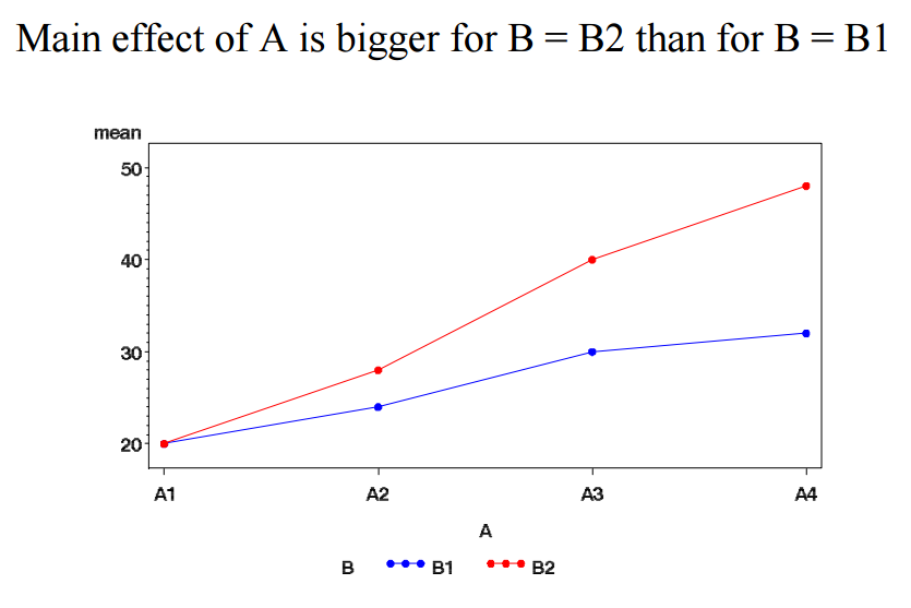
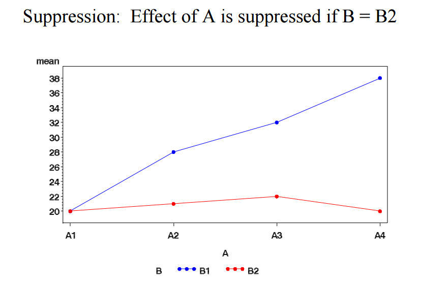
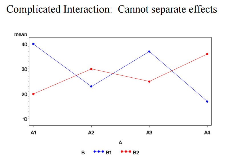
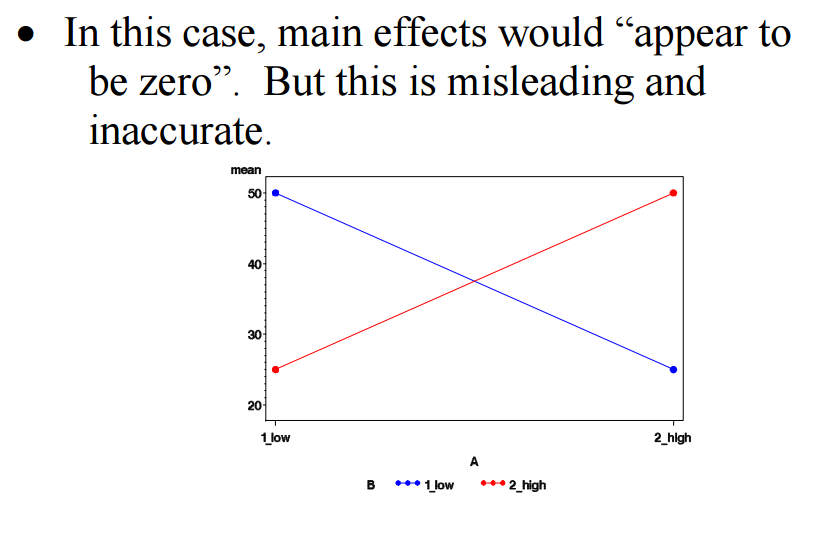
- the p-value for the interaction between supp*dose is 0.02 (significant), which indicates that the relationships between dose and tooth length depends on the supp method.
pair-wise test
> TukeyHSD(res.aov3, which = "dose")
  Tukey multiple comparisons of means
    95% family-wise confidence level

Fit: aov(formula = len ~ supp * dose, data = tdata)

$dose
        diff       lwr       upr   p adj
d1-dh  9.130  6.362488 11.897512 0.0e+00
d2-dh 15.495 12.727488 18.262512 0.0e+00
d2-d1  6.365  3.597488  9.132512 2.7e-06
pairwise.t.test(tdata$len, tdata$dose, p.adjust.method = "BH")
Homogeneity
plot(res.aov3, 1)
install.packages("car")
library(car)
leveneTest(len ~ supp*dose, data = tdata)

Levene's Test for Homogeneity of Variance (center = median)
      Df F value Pr(>F)
group  5  1.7086 0.1484
      54
p value is greater than .05, which indicates that there is no evidence of significant difference between variances of groups.
check normality
plot(res.aov3, 2)
The residuals are plotted against the quantiles of normal distribution (the straight line).
unbalance design
> library(car)
> my_anova <- aov(len ~ supp * dose, data = tdata)
>
> Anova(my_anova, type="III"
+ )
Anova Table (Type III tests)

Response: len
             Sum Sq Df F value    Pr(>F)
(Intercept) 1750.33  1 132.730 3.603e-16 ***
supp         137.81  1  10.450  0.002092 **
dose         885.26  2  33.565 3.363e-10 ***
supp:dose    108.32  2   4.107  0.021860 *
Residuals    712.11 54
---
Signif. codes:
0 ‘***’ 0.001 ‘**’ 0.01 ‘*’ 0.05 ‘.’ 0.1 ‘ ’ 1


