This is an old revision of the document!

using discrete probability distributions

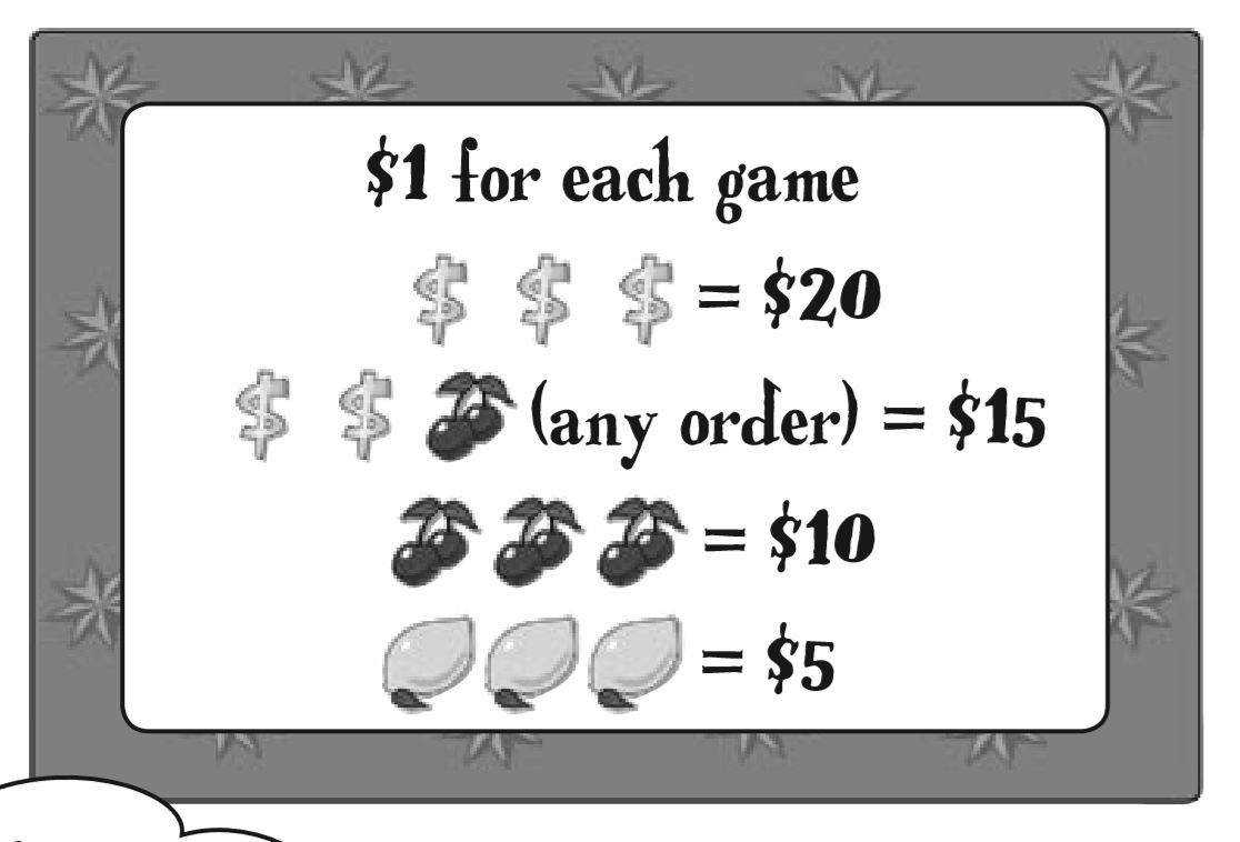
Dollar(D)	Cherry(C)	Lemon(L)	Other(O)
0.1	0.2	0.2	0.5

Probability of DDD
Probability of DDC (any order)
Probability of L
Probability of C
Probability of losing

P(D,D,D) = P(D) * P(D) * P(D)
- 0.1 x 0.1 x 0.1 = 0.001 = 1/1000

P(D,D,C) + P(D,C,D) + P(C,D,D)
- (0.1 * 0.1 * 0.2) + (0.1 * 0.2 * 0.1) + (0.2 * 0.1 * 0.1) = 6/1000

P(L,L,L) = P(L) + P(L) + P(L)
- .2 * .2 * .2 = .008 = 8/1000

P(C,C,C) = P(C) + P(C) + P(C)
- .2 * .2 * .2 = .008 = 8/1000

for nothing
- 1 - (1/1000 + 6/1000 + 8/1000 + 8/1000) = 1- 23/1000 = 977/1000

Prob. distribution

Combination	None	Lemons	Cherries	Dollars/cherry	Dollars
Probability	0.977	0.008	0.008	0.006	0.001

Combination	None	Lemons	Cherries	Dollars/cherry	Dollars
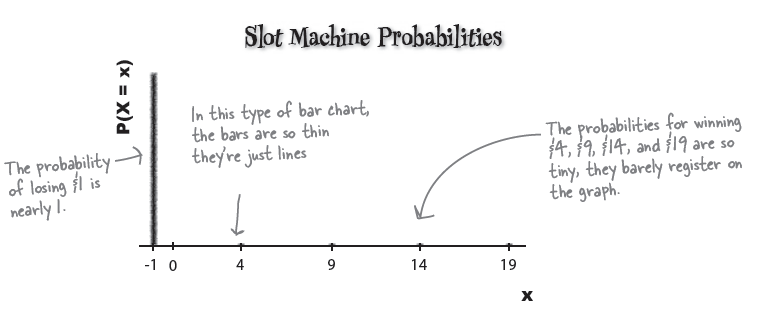
Gain	-1 dollar	4 dollar	9 dollar	14 dollar	19 dollar
Probability	0.977	0.008	0.008	0.006	0.001

Combination	None	Lemons	Cherries	Dollars/cherry	Dollars
x	-1	4	9	14	19
P(X=x)	0.977	0.008	0.008	0.006	0.001

Expectation gives you . . .

$$ E(X) = \sum{k * P(X=x)} $$

Combination	None	Lemons	Cherries	Dollars/cherry	Dollars
k	-1	4	9	14	19
P(X=x)	0.977	0.008	0.008	0.006	0.001
E(X)	-0.977	4*0.008	9**0.008	14*0.006	19*0.001

$$E(X) = -0.77$$

k <- c(-1,4,9,14,19)
Px <- c(.977,.008,.008,.006,.001)
k*Px
sum(k*Px)
exp <- sum(k*Px)
exp

> k <- c(-1,4,9,14,19)
> Px <- c(.977,.008,.008,.006,.001)
> k*Px
[1] -0.977  0.032  0.072  0.084  0.019
> sum(k*Px)
[1] -0.77
> exp <- sum(k*Px)
> exp 
[1] -0.77

Variances and probability distributions

$$E(X-\mu)^2 = \sum{(x-\mu)^2}*P(X=x) $$

$$\mu = -.77 $$

a <- c(-1,4,9,14,19)
b <- c(.977,.008,.008,.006,.001)
a*b
sum(a*b)
mu <- sum(a*b)
a-mu
(a-mu)^2
((a-mu)^2)*b
sum(((a-mu)^2)*b)
varx <- sum(((a-mu)^2)*b)

> a <- c(-1,4,9,14,19)
> b <- c(.977,.008,.008,.006,.001)
> a*b
[1] -0.977  0.032  0.072  0.084  0.019
> sum(a*b)
[1] -0.77
varx
> mu <- sum(a*b)
> a-mu
[1] -0.23  4.77  9.77 14.77 19.77
> (a-mu)^2
[1]   0.0529  22.7529  95.4529 218.1529 390.8529
> ((a-mu)^2)*b
[1] 0.0516833 0.1820232 0.7636232 1.3089174 0.3908529
> sum(((a-mu)^2)*b)
[1] 2.6971
> varx <- sum(((a-mu)^2)*b)
> varx
[1] 2.6971

Var(X) = E(X - μ)^2 * P(X=x) 
= (-1 + 0.77)^2 × 0.977 + (4 + 0.77)^2 × 0.008 
  + (9 + 0.77)^2 × 0.008 + (14 + 0.77)^2 × 0.006 
  + (19 + 0.77)^2 × 0.001
= (-0.23)^2 × 0.977 + 4.772 × 0.008 + 9.772 × 0.008 
  + 14.772 × 0.006 + 19.772 × 0.001
= 0.0516833 + 0.1820232 + 0.7636232 
  + 1.3089174 + 0.3908529
= 2.6971

Standard deviation

\begin{eqnarray*} \text{s} & = & \sqrt{s^2} \\ & = & \sqrt{2.6971} \end{eqnarray*}

> sqrt(varx)
[1] 1.642285

e.g.

Here’s the probability distribution of a random variable X:

x	1	2	3	4	5
P(X = x)	0.1	0.25	0.35	0.2	0.1

$E(X)$ ?
$Var(X) $ ?

d <- c(1,2,3,4,5)
e <- c(.1,.25,.35,.2,.1)
de <- d*e
de
sum(de)

d <- c(1,2,3,4,5)
e <- c(.1,.25,.35,.2,.1)
de <- d*e
de
sum(de)

de.mu <- sum(de)
de1 <- (d-de.mu)^2
de1

de2 <- de1*e
de2

de.var <- sum(de2)
de.var

> d <- c(1,2,3,4,5)
> e <- c(.1,.25,.35,.2,.1)
> de <- d*e
> de
[1] 0.10 0.50 1.05 0.80 0.50
> sum(de)
[1] 2.95
> 
> de.mu <- sum(de)
> de1 <- (d-de.mu)^2
> de1
[1] 3.8025 0.9025 0.0025 1.1025 4.2025
> 
> de2 <- de1*e
> de2
[1] 0.380250 0.225625 0.000875 0.220500 0.420250
> 
> de.var <- sum(de2)
> de.var
[1] 1.2475
>

> d <- c(1,2,3,4,5)
> e <- c(.1,.25,.35,.2,.1)
> de <- d*2
> de
[1]  2  4  6  8 10
> de <- d*e
> de
[1] 0.10 0.50 1.05 0.80 0.50
> sum(de)
[1] 2.95
> de.mu <- sum(de)
> de1 <- (d-de.mu)^2
> de1
[1] 3.8025 0.9025 0.0025 1.1025 4.2025
> de2 <- de1*e
> de2
[1] 0.380250 0.225625 0.000875 0.220500 0.420250
> de.var <- sum(de2)
> de.var
[1] 1.2475
>

Fat Dan changed his prices

Another probability distribution.

Combination	None	Lemons	Cherries	Dollars/cherry	Dollars
y	-2	23	48	73	98
P(Y = y)	0.977	0.008	0.008	0.006	0.001

Original one

Combination	None	Lemons	Cherries	Dollars/cherry	Dollars
k	-1	4	9	14	19
P(X=x)	0.977	0.008	0.008	0.006	0.001

k <- c(-2,   23,   48,   73,   98)
j <- c(0.977,0.008,0.008,0.006,0.001)
k*j
sum(k*j)
kj.mu <- sum(k*j)
kj.mu

> k <- c(-2,   23,   48,   73,   98)
> j <- c(0.977,0.008,0.008,0.006,0.001)
> k*j
[1] -1.954  0.184  0.384  0.438  0.098
> sum(k*j)
[1] -0.85
> kj.mu <- sum(k*j)
> kj.mu
[1] -0.85

The expectation is slightly lower, so in the long term, we can expect to lose $ 0.85 each game. The variance is
much larger. This means that we stand to lose more money in the long term on this machine, but there’s less
certainty.
Do

kj.mu <- sum(k*j)
kj.var <- sum((k-kj.mu)^2*j)
kj.var

> kj.mu <- sum(k*j)
> kj.var <- sum((k-kj.mu)^2*j)
> kj.var
[1] 67.4275
>

Q: So expectation is a lot like the
mean. Is there anything for probability
distributions that’s like the median or
mode?
A: You can work out the most likely
probability, which would be a bit like the
mode, but you won’t normally have to do this.
When it comes to probability distributions,
the measure that statisticians are most
interested in is the expectation.

Q: Shouldn’t the expectation be one of
the values that X can take?
A: It doesn’t have to be. Just as the mean
of a set of values isn’t necessarily the same
as one of the values, the expectation of a
probability distribution isn’t necessarily one
of the values X can take.

Q: Are the variance and standard
deviation the same as we had before
when we were dealing with values?
A: They’re the same, except that this time
we’re dealing with probability distributions.
The variance and standard deviation of a
set of values are ways of measuring how
far values are spread out from the mean.
The variance and standard deviation of
a probability distribution measure how
the probabilities of particular values are
dispersed.

Q: I find the concept of E(X - μ)2
confusing. Is it the same as finding
E(X - μ) and then squaring the end result?
A: No, these are two different calculations.
E(X - μ)2 means that you find the square of
X - μ for each value of X, and then find the
expectation of all the results. If you calculate
E(X - μ) and then square the result, you’ll get
a completely different answer.
Technically speaking, you’re working out
E((X - μ)2), but it’s not often written that way.

Q: So what’s the difference between a
slot machine with a low variance and one
with a high variance?
A: A slot machine with a high variance
means that there’s a lot more variability in
your overall winnings. The amount you could
win overall is less predictable.
In general, the smaller the variance is, the
closer your average winnings per game are
likely to be to the expectation. If you play on
a slot machine with a larger variance, your
overall winnings will be less reliable.

Pool puzzle

\begin{eqnarray*} X & = & (\text{original win}) - (\text{original cost}) \\ & = & (\text{original win}) - 1 \\ (\text{original win}) & = & X + 1 \\ \\ Y & = & 5 * (\text{original win}) - (\text{new cost}) \\ & = & 5 * (\text{X + 1}) - 2 \\ & = & 5 * X + 5 - 2 \\ & = & 5 * X + 3 \\ \end{eqnarray*}

E(X) = -.77 and E(Y) = -.85. What is 5 * E(X) + 3?

$ 5 * E(X) = -3.85 $
$ 5 * E(X) + 3 = -0.85 $
$ E(Y) = 5 * E(X) + 3 $

$ 5 * Var(X) = 13.4855 $
$ 5^2 * Var(X) = 67.4275 $
$ Var(Y) = 5^2 * Var(X) $

\begin{eqnarray*} E(aX + b) & = & a \cdot E(X) + b \\ Var(aX + b) & = & a^{2} \cdot Var(X) \\ E(X + Y) & = & E(X) + E(Y) \\ Var(X + Y) & = & Var(X) + Var(Y) \\ \end{eqnarray*}

\begin{eqnarray*} E(X1 + X2 + \ldots Xn) & = & nE(X) \\ Var(X1 + X2 + \ldots Xn) & = & nVar(X) \\ \end{eqnarray*}

\begin{eqnarray*} E(X + Y) & = & E(X) + E(Y) \\ Var(X + Y) & = & Var(X) + Var(Y) \\ E(X - Y) & = & E(X) - E(Y) \\ Var(X - Y) & = & Var(X) - Var(Y) \\ E(aX + bY) & = & aE(X) + bE(Y) \\ Var(aX + bY) & = & a^{2}Var(X) + b^{2}Var(Y) \\ E(aX - bY) & = & aE(X) - bE(Y) \\ Var(aX - bY) & = & a^{2}Var(X) - b^{2}Var(Y) \\ \end{eqnarray*}

A restaurant offers two menus, one for weekdays and the other for weekends. Each menu offers four set prices, and the probability distributions for the amount someone pays is as follows:

Weekday:
x	10	15	20	25
P(X = x)	0.2	0.5	0.2	0.1

Weekend:
y	15	20	25	30
P(Y = y)	0.15	0.6	0.2	0.05

Who would you expect to pay the restaurant most: a group of 20 eating at the weekend, or a group of 25 eating on a weekday?

COMMunication
RESearch.NET

Table of Contents