multicolinearity
This is an old revision of the document!
Multi-colinearity
> cps <- read.csv("http://commres.net/wiki/_media/cps_85_wages.csv", header = T, sep = "\t")
> str(cps)
'data.frame':	534 obs. of  11 variables:
 $ education : int  8 9 12 12 12 13 10 12 16 12 ...
 $ south     : int  0 0 0 0 0 0 1 0 0 0 ...
 $ sex       : int  1 1 0 0 0 0 0 0 0 0 ...
 $ experience: int  21 42 1 4 17 9 27 9 11 9 ...
 $ union     : int  0 0 0 0 0 1 0 0 0 0 ...
 $ wage      : num  5.1 4.95 6.67 4 7.5 ...
 $ age       : int  35 57 19 22 35 28 43 27 33 27 ...
 $ race      : int  2 3 3 3 3 3 3 3 3 3 ...
 $ occupation: int  6 6 6 6 6 6 6 6 6 6 ...
 $ sector    : int  1 1 1 0 0 0 0 0 1 0 ...
 $ marr      : int  1 1 0 0 1 0 0 0 1 0 ...
> head(cps)
> head(cps)
  education south sex experience union  wage age race occupation sector marr
1         8     0   1         21     0  5.10  35    2          6      1    1
2         9     0   1         42     0  4.95  57    3          6      1    1
3        12     0   0          1     0  6.67  19    3          6      1    0
4        12     0   0          4     0  4.00  22    3          6      0    0
5        12     0   0         17     0  7.50  35    3          6      0    1
6        13     0   0          9     1 13.07  28    3          6      0    0
> lm1 = lm(log(cps$wage) ~., data = cps)
> summary(lm1)

Call:
lm(formula = log(cps$wage) ~ ., data = cps)

Residuals:
     Min       1Q   Median       3Q      Max
-2.16246 -0.29163 -0.00469  0.29981  1.98248

Coefficients:
             Estimate Std. Error t value Pr(>|t|)
(Intercept)  1.078596   0.687514   1.569 0.117291
education    0.179366   0.110756   1.619 0.105949
south       -0.102360   0.042823  -2.390 0.017187 *
sex         -0.221997   0.039907  -5.563 4.24e-08 ***
experience   0.095822   0.110799   0.865 0.387531
union        0.200483   0.052475   3.821 0.000149 ***
age         -0.085444   0.110730  -0.772 0.440671
race         0.050406   0.028531   1.767 0.077865 .
occupation  -0.007417   0.013109  -0.566 0.571761
sector       0.091458   0.038736   2.361 0.018589 *
marr         0.076611   0.041931   1.827 0.068259 .
---
Signif. codes:  0 ‘***’ 0.001 ‘**’ 0.01 ‘*’ 0.05 ‘.’ 0.1 ‘ ’ 1

Residual standard error: 0.4398 on 523 degrees of freedom
Multiple R-squared:  0.3185,	Adjusted R-squared:  0.3054
F-statistic: 24.44 on 10 and 523 DF,  p-value: < 2.2e-16
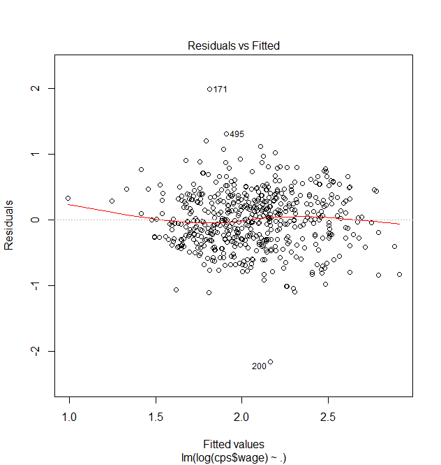
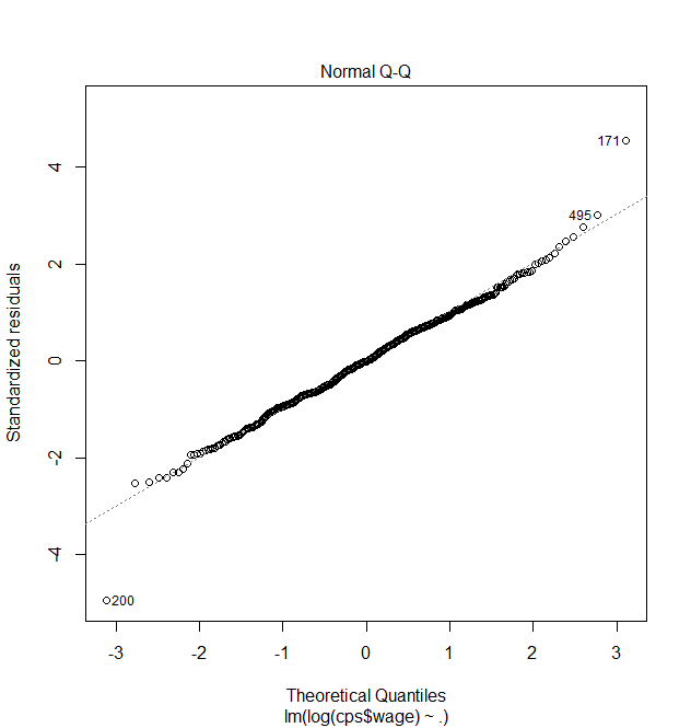
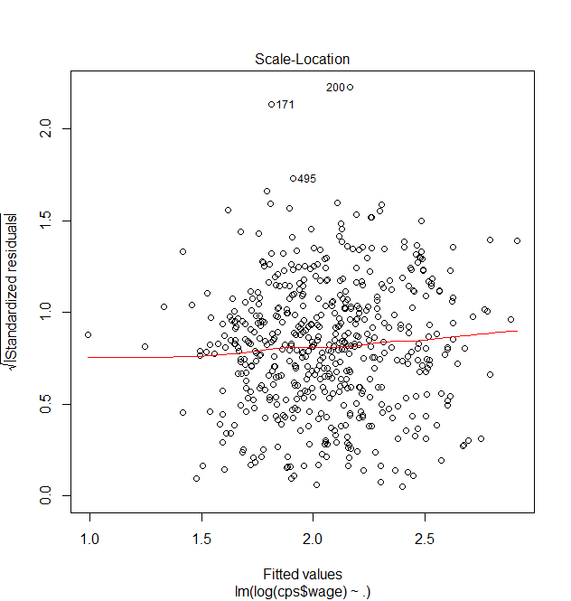
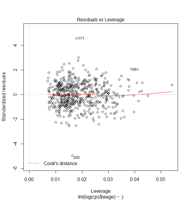
plot(lm1)
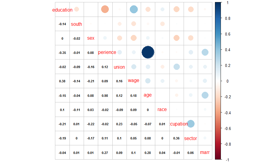
> library(corrplot)
> cps.cor = cor(cps)
> corrplot.mixed(cps.cor, lower.col = "black", number.cex = .7)
> install.packages("mctest")
> library(mctest)
> omcdiag(cps[,c(-6)], cps$wage) # or "omcdiag(cps[,c(1:5,7:11)], cps$wage)" will work as well.

Call:
omcdiag(x = cps[, c(-6)], y = cps$wage)


Overall Multicollinearity Diagnostics

                       MC Results detection
Determinant |X'X|:         0.0001         1
Farrar Chi-Square:      4833.5751         1
Red Indicator:             0.1983         0
Sum of Lambda Inverse: 10068.8439         1
Theil's Method:            1.2263         1
Condition Number:        739.7337         1

1 --> COLLINEARITY is detected by the test
0 --> COLLINEARITY is not detected by the test

>
> imcdiag(cps[,c(-6)],cps$wage)

Call:
imcdiag(x = cps[, c(-6)], y = cps$wage)


All Individual Multicollinearity Diagnostics Result

                 VIF    TOL          Wi          Fi Leamer      CVIF Klein
education   231.1956 0.0043  13402.4982  15106.5849 0.0658  236.4725     1
south         1.0468 0.9553      2.7264      3.0731 0.9774    1.0707     0
sex           1.0916 0.9161      5.3351      6.0135 0.9571    1.1165     0
experience 5184.0939 0.0002 301771.2445 340140.5368 0.0139 5302.4188     1
union         1.1209 0.8922      7.0368      7.9315 0.9445    1.1464     0
age        4645.6650 0.0002 270422.7164 304806.1391 0.0147 4751.7005     1
race          1.0371 0.9642      2.1622      2.4372 0.9819    1.0608     0
occupation    1.2982 0.7703     17.3637     19.5715 0.8777    1.3279     0
sector        1.1987 0.8343     11.5670     13.0378 0.9134    1.2260     0
marr          1.0961 0.9123      5.5969      6.3085 0.9551    1.1211     0

1 --> COLLINEARITY is detected by the test
0 --> COLLINEARITY is not detected by the test

education , south , experience , age , race , occupation , sector , marr , coefficient(s) are non-significant may be due to multicollinearity

R-square of y on all x: 0.2805

* use method argument to check which regressors may be the reason of collinearity
===================================
>
multicolinearity.1545758112.txt.gz · Last modified: by hkimscil

