Table of Contents
Normal distribution functions
| Function | Purpose |
|---|---|
| dnorm | Normal density |
| pnorm | Normal distribution function |
| qnorm | Normal quantile function |
| rnorm | Normal random variates |
Table 8-1. Discrete distributions
| Discrete distribution | R name | Parameters |
| Binomial | binom | n = number of trials; p = probability of success for one trial |
| Geometric | geom | p = probability of success for one trial |
| Hypergeometric | hyper | m = number of white balls in urn; n = number of black balls in urn; k = number of balls drawn from urn |
| Negative binomial (NegBinomial) | nbinom | size = number of successful trials; either prob = probability of successful trial or mu = mean |
| Poisson | pois | lambda = mean |
Table 8-2. Continuous distributions
| Continuous distribution | R name | Parameters |
| Beta | beta | shape1; shape2 |
| Cauchy | cauchy | location; scale |
| Chi-squared (Chisquare) | chisq | df = degrees of freedom |
| Exponential | exp | rate |
| F | f | df1 and df2 = degrees of freedom |
| Gamma | gamma | rate; either rate or scale |
| Log-normal (Lognormal) | lnorm | meanlog = mean on logarithmic scale; sdlog = standard deviation on logarithmic scale |
| Logistic | logis | location; scale |
| Normal | norm | mean; sd = standard deviation |
| Student’s t (TDist) | t | df = degrees of freedom |
| Uniform | unif | min = lower limit; max = upper limit |
| Weibull | weibull | shape; scale |
| Wilcoxon | wilcox | m = number of observations in first sample; n = number of observations in second sample |
pnorm, qnorm
Normal distribution
$ f(x) = \frac{1}{\sigma \sqrt{2\pi}} e^{\frac{-(x-\mu)^2}{2\sigma^2}} $
Assume that the test scores of a college entrance exam fits a normal distribution. Furthermore, the mean test score is 72, and the standard deviation is 15.2. What is the percentage of students scoring 84 or more in the exam?
> pnorm(72, mean=72, sd=15.2, lower.tail=FALSE)
[1] 0.5

> pnorm(1.96)
[1] 0.9750021

> pnorm(1.96)-pnorm(-1.96)
[1] 0.9500042

> pnorm(c(1.96, -1.96))
[1] 0.9750021 0.0249979

> pnorm(84, mean=72, sd=15.2, lower.tail=FALSE)
[1] .2149176

> qnorm(.2149176, mean=72, sd=15.2, lower.tail=FALSE)
[1] 84
rnorm
Random samples from a normal distribution
> set.seed(1024)
> rnorm(50)
 [1] -0.778662882 -0.389476396 -2.033798329 -0.982373104  0.247890054
 [6] -2.103864629 -0.381418049  2.074919838  1.027138407  0.473014228
[11] -1.879263193 -1.239189026  1.160418602  0.003671291 -0.095452066
[16]  1.795551228 -1.322138481 -0.276086413 -0.743976510 -1.070050125
[21] -0.349525474  0.805559661  1.605301660  1.447595754 -0.128302224
[26] -0.538926447  0.391586050  0.879217023 -0.824732092  0.732876423
[31] -0.664914510  0.360885549  1.011930957 -0.235916848  1.353589893
[36] -0.268632965  1.019877368 -0.279706500 -0.618146278 -0.499273059
[41] -0.153716777  1.220869694 -0.669570510 -1.209660342  1.024096655
[46]  0.603955311 -0.568653469 -0.891303117 -2.525145692  0.589357049
qt, pt
$t = \frac{Z}{\sqrt{\frac{V}{m}}}$
> qt(c(0.025, 0.975), df=5)
[1] -2.5706  2.5706

> qt(c(0.025, 0.975), df=10)
[1] -2.228139  2.228139

> qt(c(0.025, 0.975), df=20)
[1] -2.085963  2.085963

> qt(c(0.025, 0.975), df=30)
[1] -2.042272  2.042272

> qt(c(0.025, 0.975), df=40)
[1] -2.021075  2.021075

> qt(c(0.025, 0.975), df=50)
[1] -2.008559  2.008559

. . . . . .

> qt(c(0.025, 0.975), df=50000)
[1] -1.960011  1.960011
Counting the Number of Combinations
A common problem in computing probabilities of discrete variables is counting combinations: the number of distinct subsets of size k that can be created from n items. The number is given by
$$n!/r!(n − r)!$$
But it’s much more convenient to use the choose function—especially as n and k grow larger:
> choose(5,3)       # How many ways can we select 3 items from 5 items?
[1] 10
> choose(50,3)      # How many ways can we select 3 items from 50 items?
[1] 19600
> choose(50,30)     # How many ways can we select 30 items from 50 items?
[1] 4.712921e+13
These numbers are also known as binomial coefficients.
Generating Combinations
> combn(1:5,3)
     [,1] [,2] [,3] [,4] [,5] [,6] [,7] [,8] [,9] [,10]
[1,]    1    1    1    1    1    1    2    2    2     3
[2,]    2    2    2    3    3    4    3    3    4     4
[3,]    3    4    5    4    5    5    4    5    5     5
The function is not restricted to numbers. We can generate combinations of strings, too. Here are all combinations of five treatments taken three at a time:
> combn(c("T1","T2","T3","T4","T5"), 3)
     [,1] [,2] [,3] [,4] [,5] [,6] [,7] [,8] [,9] [,10]
[1,] "T1" "T1" "T1" "T1" "T1" "T1" "T2" "T2" "T2" "T3"
[2,] "T2" "T2" "T2" "T3" "T3" "T4" "T3" "T3" "T4" "T4"
[3,] "T3" "T4" "T5" "T4" "T5" "T5" "T4" "T5" "T5" "T5"
Generating Random Numbers
The simple case of generating uniform random numbers between 0 and 1 is handled by the runif function:
> runif(1)
[1] 0.5119812
Generating a vector of 10 such values:
> runif(10)
 [1] 0.03475948 0.88950680 0.90005434 0.95689496 0.55829493 0.18407604
 [7] 0.87814788 0.71057726 0.11140864 0.66392239
> runif(1, min=-3, max=3)          # One uniform variate between -3 and +3
[1] 2.954591
> rnorm(1)                         # One standard Normal variate
[1] 1.048491
> rnorm(1, mean=100, sd=15)        # One Normal variate, mean 100 and SD 15
[1] 108.7300
> rbinom(1, size=10, prob=0.5)     # One binomial variate
[1] 3
> rpois(1, lambda=10)              # One Poisson variate
[1] 13
> rexp(1, rate=0.1)                # One exponential variate
[1] 8.430267
> rgamma(1, shape=2, rate=0.1)     # One gamma variate
[1] 20.47334
> rnorm(3, mean=c(-10,0,+10), sd=1) # mean이 각 -10,0,10이고 각 mean의 sd가 1인 경우에, random score를 구할것
[1] -11.195667   2.615493  10.294831
Recycling the vector . . .
> rnorm(6, mean=c(-10,0,+10), sd=1)
[1] -11.74168122   0.56572232  11.88595452 -11.13726844
[5]   0.03274875   9.02216868
Generating Reproducible Random Numbers
After generating random numbers, you may often want to reproduce the same sequence of “random” numbers every time your program executes.
> set.seed(165)          # Initialize the random number generator to a known state
> runif(10)              # Generate ten random numbers
 [1] 0.1159132 0.4498443 0.9955451 0.6106368 0.6159386 0.4261986 0.6664884
 [8] 0.1680676 0.7878783 0.4421021
> set.seed(165)          # Reinitialize to the same known state
> runif(10)              # Generate the same ten "random" numbers
 [1] 0.1159132 0.4498443 0.9955451 0.6106368 0.6159386 0.4261986 0.6664884
 [8] 0.1680676 0.7878783 0.4421021
Generating a Random Sample
Suppose your World Series data contains a vector of years when the Series was played. You can select 10 years at random using sample:
year <- c(1900:2016)     # years in vector year
world.series <- data.frame(year)
> sample(world.series$year, 10)
 [1] 1906 1963 1966 1928 1905 1924 1961 1959 1927 1934
The items are randomly selected, so running sample again (usually) produces a different result:
> sample(world.series$year, 10)
 [1] 1968 1947 1966 1916 1970 1961 1936 1913 1914 1958
Replacement in random sampling: Specify replace=TRUE to sample with replacement.
> set.seed(121)
sample(world.series$year, 10)
 [1] 1906 1963 1966 1928 1905 1924 1961 1959 1927 1934
set.seed(121)
sample(world.series$year, 10)
 [1] 1906 1963 1966 1928 1905 1924 1961 1959 1927 1934
Generating Random Sequences
> sample(set, n, replace=TRUE)

> sample(c("H","T"), 10, replace=TRUE)
 [1] "H" "H" "H" "T" "T" "H" "T" "H" "H" "T"

> sample(c(FALSE,TRUE), 20, replace=TRUE)
 [1]  TRUE FALSE FALSE FALSE FALSE FALSE FALSE  TRUE  TRUE  TRUE  TRUE  TRUE
[13]  TRUE  TRUE FALSE  TRUE  TRUE FALSE FALSE  TRUE
> sample(c(FALSE,TRUE), 20, replace=TRUE, prob=c(0.2,0.8))
 [1]  TRUE  TRUE  TRUE  TRUE  TRUE  TRUE  TRUE FALSE  TRUE  TRUE  TRUE  TRUE
[13]  TRUE  TRUE  TRUE  TRUE  TRUE  TRUE FALSE  TRUE
Randomly Permuting a Vector
> sample(1:10)
 [1]  5  8  7  4  3  9  2  6  1 10
Calculating Probabilities for Continuous Distributions
| Distribution | Distribution function: P(X ≤ x) |
| Normal | pnorm(x, mean, sd) |
| Student’s t | pt(x, df) |
| Exponential | pexp(x, rate) |
| Gamma | pgamma(x, shape, rate) |
| Chi-squared (χ2) | pchisq(x, df) |
> pnorm(66, mean=70, sd=3)
[1] 0.09121122
> pnorm(73, mean=70, sd=3)
[1] ??
> b <- pnorm(-1)
> a <- pnorm(1)
> a-b
[1] 0.6826895

> b <- pnorm(-2)
> a <- pnorm(2)
> a-b
[1] 0.9544997

> a <- pnorm(3)
> b <- pnorm(-3)
> a-b
[1] 0.9973002
> b <- pnorm(-1.959964)
> a <- pnorm(1.959964)
> a-b
[1] 0.95
Converting Probabilities to Quantiles
> qnorm(0.8413447, mean=70, sd=3)
[1] 73
> pnorm(73, mean=70, sd=3)
[1] 0.8413447
> qnorm(c(0.025, 0.975)) # 5% 바깥쪽의 점수는 약 +-2sd 점수인 -2, 2
[1] -1.959964  1.959964
Plotting a Density Function
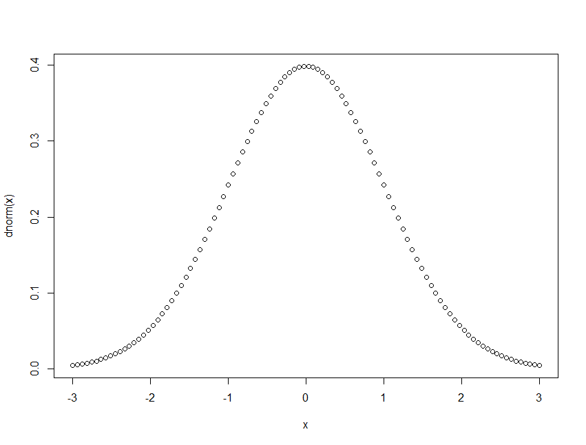
> x <- seq(from=-3, to=+3, length.out=100)
> plot(x, dnorm(x))
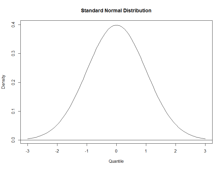
> x <- seq(from=-3, to=+3, length.out=100)
> y <- dnorm(x)
> plot(x, y, main="Standard Normal Distribution", type='l',
+      ylab="Density", xlab="Quantile")
> abline(h=0)
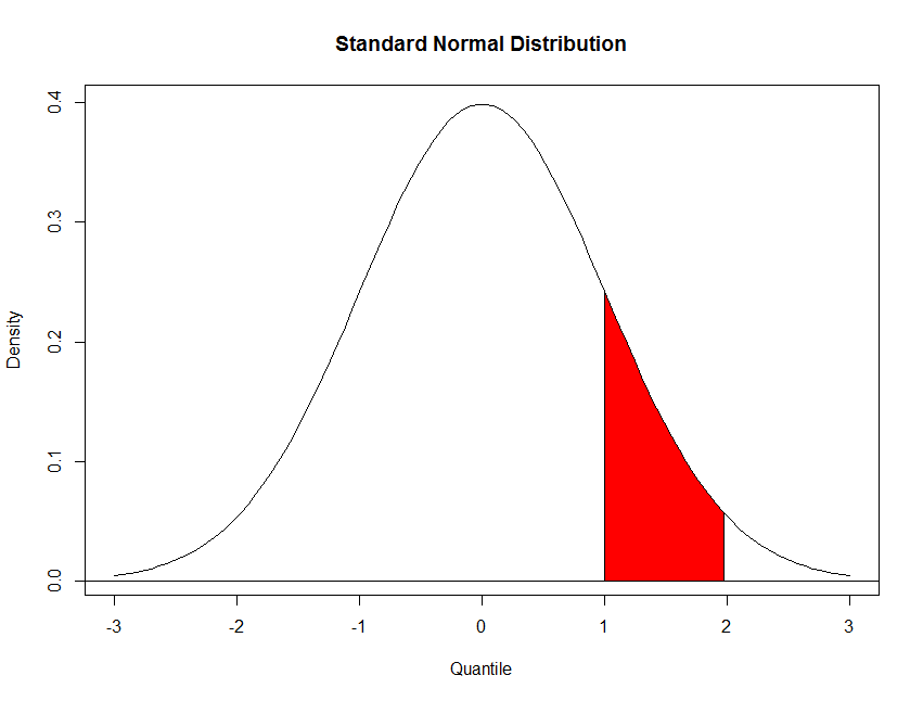
> # The body of the polygon follows the density curve where 1 <= z <= 2
> region.x <- x[1 <= x & x <= 2]
> region.y <- y[1 <= x & x <= 2]
>
> # We add initial and final segments, which drop down to the Y axis
> region.x <- c(region.x[1], region.x, tail(region.x,1))
> region.y <- c(          0, region.y,                0)
> polygon(region.x, region.y, density=-1, col="red")


