Table of Contents
요인분석
fa_explanation.csv
saq.csv
efa.csv
In order to understand factor analysis, you should understand how regression coefficients work, how they are interpreted. Therefore, please review variance, regression R square value, regression coefficient, beta, etc.
- 다수의 변수들 간의 상호관련성을 소수의 요인(factor)으로 정리하는 방법의 하나로 전체 변수에 공통적인 요인이 있다고 가정하고 (예, 30개의 질문이 동일한 무엇인가를 묻고 있기 때문에 서로 상관관계가 있을 것)
- 이 요인을 찾아내어 각 변수가 어느 정도 영향을 받고 있는지 그 정도를 산출하기도 하고 그 집단의 특성이 무엇인가를 기술하려는 통계기법
- 질문 문항들, 변수들 혹은 측정 대상들간의 상관관계를 고려해서 이들 측정치 사이에 공유하는 구조를 파악해 내는 기법을 말함
- 변수의 숫자를 요인으로 줄이는 기법으로 변수가 독립변수/ 종속변수인가를 구분하지 않음
- See e.g. 1 example

d = read.table("http://commres.net/wiki/_media/r/personality0.txt")
saq.csv file은 아래 설문조사에 대한 데이터로서 총 2571명이 응답하였다. 위의 설명이 어려운것 같지만, 간단히 이야기하면 응답자들이 대답한 것들에 대한 공통적인 요인을 추출하게 되면 여러가지의 질문이 몇가지의 요인으로 구분되어 있다고 주장할 수 있게 된다는 뜻이다. 가령 아래의 질문들이 우리가 눈으로 봐서 4개의 요인을 묻는 질문이라고 생각할 수 있다.
- 컴퓨터 사용에 대한 태도
- 통계에 (statistics) 태도
- 수학에 대한 태도
- 통계페키지 프로그램에 (SPSS) 대한 태도
얼뜻 눈으로 이 4개의 요인을 (혹은 단면, 측면, dimensions) 뽑아냈지만 응답자들의 응답에 섞인 상관관계에 기초하여 이런 요인들을 추출해 낼 수 있다면 좋겠는데 이것이 요인분석이 (factor analysis) 하는 일이다. 어떤 응답자가 수학이 싫은면 수학과 관련된 어떤 질문들에 대해서 비슷한 (상관관계가 높게) 답변을 할 것이니 가능한 것이다.
Questionnaire:
- Statiscs makes me cry
- My friends will think I'm stupid for not being able to cope with SPSS
- Standard deviations excite me
- I dream that Pearson is attacking me with correlation coefficients
- I don't understand statistics
- I have little experience of computers
- All computers hate me
- I have never been good at mathematics
- My friends are better at statistics than me
- Computers are useful only for playing games
- I did badly at mathematics at school
- People try to tell you that SPSS makes statistics easier to understand but it doesn't
- I worry that I will cause irreparable damage because of my incompetenece with computers
- Computers have minds of their own and deliberately go wrong whenever I use them
- Computers are out to get me
- I weep openly at the mention of central tendency
- I slip into a coma whenever I see an equation
- SPSS always crashes when I try to use it
- Everybody looks at me when I use SPSS
- I can't sleep for thoughts of eigen vectors
- I wake up under my duvet thinking that I am trapped under a normal distribtion
- My friends are better at SPSS than I am
- If I'm good at statistics my friends will think I'm a nerd
목적
- 자료의 요약: 여러 개의 변인들을 몇 개의 공통된 집단으로 묶음으로써 자료의 복잡성 줄이고 정보를 요약하는데 이용
- 아이디어, 구성1)의 구조파악: 동질적인 변인들을 몇 개의 요인들로 묶어줌으로써 변인들 내에 존재하는 상호 독립적인 특성을 발견하는데 이용
- 불필요한 변인의 제거: 변인군으로 묶이지 않은 변인을 제거함으로써 중요하지 않은 변인 선별가능
- 측정도구의 타당성 검증: 동일한 개념을 측정한 변인들이 동일한 요인으로 묶이는지 여부 확인함으로써 측정도구 타당성을 검증하는데 이용
요건
- 숫자 측정 변수 (interval, ratio)
- data 정규분포
- 상호독립적 개인
- 등분산
- 표본 수: 최소한 50이상, 100넘는 것이 정상/ 일반적으로 변수수의 4-5배(보수적), ), 경우에 따라서 2배
Example
| 학생 no. | 시험 점수 : | ||
|---|---|---|---|
| 회계(finance), Y1 | 마케팅(marketing), Y2 | 정책(policy), Y3 |
|
| 1 | 3 | 6 | 5 |
| 2 | 7 | 3 | 3 |
| 3 | 10 | 9 | 8 |
| 4 | 3 | 9 | 7 |
| 5 | 10 | 6 | 5 |
학생들의 점수가 위와 같다고 하고, 이 점수는 사실은 두 가지 잠재적인 요인에 의해서 결정되는 것이라고 하자. 이 두 가지 잠재적 요인은 수적능력과 (quantitative) 언어적능력이다 (verbal).
각 과목의 점수는 위의 가정을 받아들인다면 아래와 같은 regression으로 정리할 수 있다.
\begin{equation} \label{eq1} \begin{split} Y_{1} &= \beta_{10} + \beta_{11}F_{1} + \beta_{12}F_{2} + e_{1} \\ Y_{2} &= \beta_{20} + \beta_{21}F_{1} + \beta_{22}F_{2} + e_{2} \\ Y_{3} &= \beta_{30} + \beta_{31}F_{1} + \beta_{32}F_{2} + e_{3} \end{split} \end{equation}
위 식 $(1)$에서 $e_{i}$는 error term을 말하고, $F1$, $F2$ 는 각각 잠재적인 요인이다. finance $(Y_{1})$, marketing $(Y_{2})$, policy $(Y_{3})$ 점수는 $F1$과 $F2$의 기여로 만들어지는 점수이다. $F1$과 $F2$가 observation에 기초한 변인이 아니므로 데이터를 이용한 regression을 구하는 방법은 적당치 않다. 따라서 다른 방법으로 이를 해결해야 한다.
한편, $\beta_{ij}$ 는 표준화된 correlation coefficient 값을 말한다 (regression에서 beta값) – factor analysis에서는 흔히 factor loading이라고 부른다. beta를 해석하는 방법과 마찬가지로 factor loading 값은 F1이나 F2의 인자가 finance (혹은 다른 변인 점수, $Y_{i}$) 점수에 얼마나 기여하는지를 나타내 주는 지표라고 하겠다.
상식을 이용해서 문제를 살펴보면, finance 시험은 숫적능력과 관련이 있으므로 $F1$ 앞에 (이름을 붙이면 숫적능력) 붙는 $\beta_{ij}$값이 (factor loading 값이) 커야하는 것이 이치라고 하겠고, 반대로 Marketing과 Policy시험은 언어능력의 요인($F2$)의 loading값이 커야 하겠다 (아래 표 참조).
| Loadings on: | ||
|---|---|---|
| Variable $Y_{i}$ | $F_{1},\,\,\beta_{i1}$ 숫적능력 | $F_{2},\,\,\beta_{i2}$ 언어능력 |
| $Y_{1}$ 회계 | + | 0 |
| $Y_{2}$ 마케팅 | 0 | + |
| $Y_{3}$ 정책 | 0 | + |
위의 요인이 포함된 regression공식이 갖는 가정은 다음과 같다.
- $E(e_{i}) = 0, \quad Var(e_{i}) = \sigma^2_{i}$
- error의 분포에 관한 내용이다.
- expected value = mean of error terms = 0, with standard deviation = $\sigma_{i}$
- 에러는 평균 0을 중심으로 무작위로 펼쳐져 있는 상태가 가정되므로 위와 같은 성격을 갖는다.
- $E(F_{j}) = 0, \quad Var(F_{j}) = 1 $
- F는 표준화된 coefficient로 크기가 나타내지는 가상의 인자이다 (factor).
- Factors are standardized with mean =0, standard deviation = 1. Hence, Var(F) = 1.
- factors의 계수를 내기 전의 data는 표준점수 처리가 된 것을 가정한다. 따라서, F의 mean과 standard deviation값은 각각 0과 1이어야 하고, 따라서 F의 variance값 또한 1이 된다.
한편, variance와 covariance의 성질은 다음과 같다 (Rules of Variance and Covariance in Statistical Review). 이를 바탕으로 아래의 Factor가 사용된 regression공식에서 각 변인의 variance 값을 살펴보자면,
$$Y_{i} = \beta_{i0} + \beta_{i1}F_{1} + \beta_{i2}F_{2} + (1) e_{i} $$
\begin{align*} Var(Y_i) & = \beta^2_{i1}Var(F1) + \beta^2_{i2}Var(F2) + (1)^2Var(e_i) \\ & = \underbrace{ \;\beta^2_{i1} \qquad\quad\;\; + \beta^2_{i2} }_\text{communality} \qquad\quad\;\; + \quad \underbrace{ \sigma^2_{i} }_\text{specific variance} \end{align*}
Variance 성질에 따라서 우리는 다음을 도출할 수 있다.
- $\beta_{i0}$는 상수(constant)이므로 0,
- $F1$, $F2$ 의 분산값은 1이고, coefficient값은 $F1$ 요인에 곱한 상수이므로 분산을 구하기 위해서는 제곱을 해야 한다. 따라서, $F1$ $F2$에 해당하는 분산값은 각각 $\beta^2_{i1} + \beta^2_{i2}$
- error term의 분산값은 위 가정에서 언급된 것처럼 $\sigma^2_{i}$
- 이를 해석하자면,
- fiance (혹은 다른 시험) 점수의 총 분산값은 $F1$과 $F2$의 coefficient(loading)값을 각각 제곱해서 더한 것에
- 에러의 분산값을 더한 것과 같다.
- 여기서 loading 제곱의 합은 regression으로 설명되는 부분이고
- 에러의 분산값은 어느 factor에도 기여를 하지 못하는 나머지 부분이다.
- 즉, fiance의 분산값은 $F1$, $F2$가 기여하는 부분과 이 둘에 포함되지 않는 나머지로 나눌 수 있다. 이는 regression에서 explained(regression) variance와 unexplained variance를 이야기 하는 것과 같은 이치이다.
- 앞의 두 coefficient(계수 혹은 factor loading)을 communality라고 부른다. 이 이름이 자연스러운 것은 Y의 총분산 중 두 요인($F1$, $F2$)이 공통적으로 기여하는 부분의 분산이기 때문이다.
- 따라서, 마지막 에러텀에 해당하는 분산은 specific variance라고 이름을 붙히는 것이 자연스럽다. 즉, Y의 총 분산 중 어느 요인에게도 영향을 받지 않는 나머지 즉, 공통적(communality)인 것에서 specific한 분산의 부분이다.
이를 covariance matrix에 정리하자면 아래와 같다.
| Variable | Y1 | Y2 | Y3 |
| Y1 | $\beta^2_{11} + \beta^2_{12} + \sigma^2_{1}$ | ||
| Y2 | $\beta^2_{21} + \beta^2_{22} + \sigma^2_{2}$ | ||
| Y3 | $\beta^2_{31} + \beta^2_{32} + \sigma^2_{3}$ |
한편, 두 변인 (가령, fiance점수와 marketing점수) 간의 covariance를 구하는 것과 관련해서는:
\begin{align*} Y_{i} & = \beta_{i0} + \beta_{i1}F1 + \beta_{i2}F2 + (1)e_{i} + (0)e_{j} \\ Y_{j} & = \beta_{j0} + \beta_{j1}F1 + \beta_{j2}F2 + (0)e_{i} + (1)e_{j} \\ Cov(Y_{i}, Y_{j}) & = \beta_{i1}\beta_{j1}Var(F1) + \beta_{i2}\beta_{j2}Var(F2) + (1)(0)Var(e_{i}) + (0)(1)Var(e_{i}) \\ & = \beta_{i1} \beta_{j1} + \beta_{i2} \beta_{j2} \end{align*}
위에서
- $Cov(\beta_{i0}, \beta_{j0}) = 0 $ 둘 다 상수이므로
- (6)과 (8)에 의해서, $\beta_{i1}F1$ 와 $\beta_{j1}F1$ 간의 Covariance는 $\beta_{i1}\beta_{j1}Var(F1)$
- 그리고 위는 Var(F1) = 1이므로 $\beta_{i1}\beta_{j1}Var(F1) = \beta_{i1}\beta_{j1}$
- $Y_i$ 의 error 경우 $e_{i}$을 가지고 있고 $e_{j}$가 없으므로 $(1)e_{i} + (0)e_{j}$와 같이 표현
- $Y_j$ 의 error 경우는 $e_{j}$을 가지고 있고 $e_{i}$가 없으므로 $(0)e_{i} + (1)e_{j}$와 같이 표현
- 이제 두 error간의 Covariance는 (6)에 의해서 상수 간의 곱셈이 0이므로 0이 되어버림
이에 따라서 covariance matrix를 채워보면 아래와 같다.
| Variable | Y1 | Y2 | Y3 |
| Y1 | $\beta_{21}\beta_{11} + \beta_{22}\beta_{12}$ | $\beta_{31}\beta_{11} + \beta_{32}\beta_{12}$ | |
| Y2 | $\beta_{11}\beta_{21} + \beta_{12}\beta_{22}$ | $\beta_{21}\beta_{31} + \beta_{22}\beta_{32}$ | |
| Y3 | $\beta_{11}\beta_{31} + \beta_{12}\beta_{32}$ | $\beta_{21}\beta_{31} + \beta_{22}\beta_{32}$ |
이제 이 둘을 합치면 온전한 covariance matrix를 구할 수가 있고, 이를 Theoretical covariance matrix라고 부른다.
| Variable | Y1 | Y2 | Y3 |
| Y1 | $\beta^2_{11} + \beta^2_{12} + \sigma^2_{1}$ | $\beta_{21}\beta_{11} + \beta_{22}\beta_{12}$ | $\beta_{31}\beta_{11} + \beta_{32}\beta_{12}$ |
| Y2 | $\beta_{11}\beta_{21} + \beta_{12}\beta_{22}$ | $\beta^2_{21} + \beta^2_{22} + \sigma^2_{2}$ | $\beta_{21}\beta_{31} + \beta_{22}\beta_{32}$ |
| Y3 | $\beta_{11}\beta_{31} + \beta_{12}\beta_{32}$ | $\beta_{21}\beta_{31} + \beta_{22}\beta_{32}$ | $\beta^2_{31} + \beta^2_{32} + \sigma^2_{3}$ |
위의 covariance 테이블은 이론에 기초해서 추출한 것이다. 한편, 실제 데이터에서 covariance table을 추출해 볼 수 있는데, 이은 아래와 같이 표현된다. 테이블의 대각선은 각 Y의 분산(variance)이고, 나머지 셀은 각 변인 간의 공분산(covariance)을 적어 놓은 것이다.
| Variable | Y1 | Y2 | Y3 |
| Y1 | $S^2_{1}$ | $S_{12}$ | $S_{13}$ |
| Y2 | $S_{21}$ | $S^2_{2}$ | $S_{23}$ |
| Y3 | $S_{31}$ | $S_{32}$ | $S^2_{3}$ |
실제 데이터에서 구한 variance covariance table은 아래와 같다2).
| Variable | Y1 | Y2 | Y3 |
| Y1 | 9.84 | -0.36 | 0.44 |
| Y2 | -0.36 | 5.04 | 3.84 |
| Y3 | 0.44 | 3.84 | 3.04 |
실제 데이터로 구한 covariance matrix (가).
## 예를 들어
fd <- read.csv("http://commres.net/wiki/_media/r/fa_explanation.csv")
fd <- fd[, -1] # 처음 id 컬럼 지우기
cov(fd)
$$ \begin{pmatrix} 9.84 & -0.36 & 0.44 \\ -0.36 & 5.04 & 3.84 \\ 0.44 & 3.84 & 3.04 \end{pmatrix} $$
아래는 설명한 것과 같이 이론적으로 구한 covariance matrix 이다 (나).
$$
\begin{pmatrix}
\beta^2_{11} + \beta^2_{12} + \sigma^2_{1} & \beta_{21}\beta_{11} + \beta_{22}\beta_{12} & \beta_{31}\beta_{11} + \beta_{32}\beta_{12} \\
\beta_{11}\beta_{21} + \beta_{12}\beta_{22} & \beta^2_{21} + \beta^2_{22} + \sigma^2_{2} & \beta_{21}\beta_{31} + \beta_{22}\beta_{32} \\
\beta_{11}\beta_{31} + \beta_{12}\beta_{32} & \beta_{21}\beta_{31} + \beta_{22}\beta_{32} & \beta^2_{31} + \beta^2_{32} + \sigma^2_{3}
\end{pmatrix}
$$
실제 데이터에서 구한 variance covariance 값과 (위에서 가) factor 분석에 기반한 이론 적인 variance covariance 테이블을 (위에서 나) 비교해 볼 수 있다. 이를 통해서 각 Factor의 $\beta_{ij}$ laoding 값을 유추해 볼 수 있을 것이다. Regression방법은 F1과 F2가 observed된 변인이 아니기에 할 수가 없었고, 위의 방법으로 Beta값들을 구한다면 각 요인(factor)에 대한 beta값을 바탕으로 변인들에 대한 regression공식을 완성할 수 있게 된다.
Interpretation of factor loading and the rotation method
위의 분석작업을 통해서 아래와 같은 regression 공식을 얻었다고 가정하자 (Linear Algera를 대학교육에서 가르치는 이유를 여기서도 알게된다. 그리고 거기서 배우는 Eigen vector, Eigen value 등이 지금 여기서와 무슨관계인지도. . . 그러나, 수학을 잘 모르는 학생들을 위한 설명이기에 이를 이용하지 않고 설명한다). 아래 공식의 문제점은 F1과 F2의 loading값이 골고루 퍼져 있어서, finance 점수에 영향을 주는 것이 F1인지 F2인지 이야기하기기 어렵다는 점이다. 즉, factor loadings are not unique하다는 것이다.
좀 더 설명하자면 우리가 regression에서 배운 것에 의하면 아래는 $Y_{1}$ 은 F1이 0.5만큼 F2가 0.5만큼 설명한다고 하겠다. 이것을 팩터로딩이 팩터 간에 독립적으로 나타나지 않는다고 이야기 한다는 뜻이다. 그러나 우리가 factor analysis 를 하는 이유는 Factor 중의 하나가 $Y_{1}$에 온전히 기여를 하고 나머지는 기여를 하지 않는 구조를 가지는가를 보기 위해서다. 이를 위해서 아래의 해는 로테이션이라는 과정을 한번 더 거치게 된다 (바로 아래 문장 참조 - “한편 아래의 공식에서 . . .” ).
Model A
\begin{eqnarray*}
Y_{1} =& 0.5 F1 + 0.5 F2 + e_{1} \\
Y_{2} =& 0.3 F1 + 0.3 F2 + e_{2} \\
Y_{3} =& 0.5 F1 - 0.5 F2 + e_{3} \\
\end{eqnarray*}
위의 공식을 토대로 아래와 같은 variance covariance matrix를 구해 볼 수 있다. 이는
\begin{align*}
\text{Var}_\text{(Y1)} & = (0.5)^2 + (0.5)^2 + \sigma^2_{1} \\
& = 0.5 + \sigma^2_{1} \\
\text{Cov}_\text{(Y1, Y2)} & = (0.5)(0.3) + (0.5)(0.3) \\
& = 0.3
\end{align*}
과 같은 방법으로 구한 것이다.
| Variable | Y1 | Y2 | Y3 |
| Y1 | 0.5 + $\sigma^2_{1}$ | 0.3 | 0.5 |
| Y2 | 0.3 | 0.18 + $\sigma^2_{2}$ | 0.3 |
| Y3 | 0.5 | 0.3 | 0.5 + $\sigma^2_{3}$ |
한편 아래의 공식에서 또한 이론적인 variance covariance matrix를 구해볼 수 있는데, 이는 위의 theoretical variance covariance 매트릭스와 동일한 것이다.
Model B
\begin{align*}
Y_{1} & = (\sqrt{2}/{2}) F1 + 0 F2 + e_{1} \\
Y_{2} & = (0.3\sqrt{2}) F1 + 0 F2 + e_{2} \\
Y_{3} & = 0 F1 - (\sqrt{2}/2) F2 + e_{3} \\
\end{align*}
즉,
\begin{align*}
Var(Y_{1}) & = ({\sqrt2}/{2})^2 + (0)^2 = 0.5 \\
Cov(Y_{1}, Y_{2}) & = (\sqrt2/2) * (0.3\sqrt2) = 0.3 \\
\end{align*}
등을 통해서 구한 matrix는 위의 theoretical variance covariance 매트릭스와 동일한 내용을 같는다.
그런데, 모델 B는 모델 A의 loading값에 “로테이션 방법“을 적용해서 구한 것이다. 이는 아래의 그림에서 설명이 된다. 이 그림에서 첫 번째 것은 모델 A의 loading값(coefficient값)을 좌표에 옮긴 것이다. 만약에 좌표(0.3, 0.3)을 관통하는 선을 그은 후, 이 선을 왼 쪽으로 (혹은 오른 쪽으로 돌려도 마찬가지이다) 돌려서 (rotatation이란 말은 여기서 나온 것이다) y축에 일치 시키면, y축에 일치하는 좌표의 coordinate는 이제 ($0, 0.3\sqrt2$)이 될 것이다. 같은 방법으로 다른 점들 또한 회전을 시키면 그림의 d가 보여주는 coordinate를 갖게 될 것이다. 이는 물론, 모델 B의 loading 값들이다. 즉, 모델 A와 모델 B는 동일한 threoretical covariance 테이블을 공유한다는 것이다.
이 방법은 이제 해석에서 진가를 발휘한다. 즉, 모델 B의 loading값들은 이제 F1 혹은 F2의 영향력만이 표현이 된 것이이다. 따라서, Y1은 이제 F1만의 영향을 받는다고 이야기할 수 있다 ($\beta$ 값인 $(\sqrt2/2)$ 만큼). Y2 또한 F1의 영향력만을 갖는다고 볼 수 있으며, Y3는 F1이 아닌 F2의 영향력을 받는다고 할 수 있다. 이를 토대로 이제 우리는 Y 변인들 (1,2,3)은 F1과 F2의 잠재적인 요인들로 나뉘어 질 수 있다고 주장할 수 있다.

Factor solution among many . . .
| Variable, Yi | Observed variance, S2i | Communality, $\beta^2_{i1} +\beta^2_{i2} $ |
| Finance, Y1 | S21 | $\beta^2_{11} +\beta^2_{12} $ |
| Marketing, Y2 | S22 | $\beta^2_{21} +\beta^2_{22} $ |
| Policy, Y3 | S23 | $\beta^2_{31} +\beta^2_{32} $ |
| total | Tobserved | Ttotal |
각 변인의 Observed Variance는 df (즉, n-1)을 사용하는 대신 n을 사용하여 구함.
fd <- read.csv("http://commres.net/wiki/_media/r/fa_explanation.csv")
m.fin <- mean(fd$finance)
m.mar <- mean(fd$marketing)
m.pol <- mean(fd$policy)
fin <- fd$finance
mar <- fd$marketing
pol <- fd$policy
n.fin <- length(fin)
n.mar <- length(mar)
n.pol <- length(pol)

sum((fin-m.fin)^2)/(n.fin) # variance of finance
sum((mar-m.mar)^2)/(n.mar) # variance of marketing
sum((pol-m.pol)^2)/(n.pol) # variance of policy
> fd <- read.csv("http://commres.net/wiki/_media/r/fa_explanation.csv")
> m.fin <- mean(fd$finance)
> m.mar <- mean(fd$marketing)
> m.pol <- mean(fd$policy)
> fin <- fd$finance
> mar <- fd$marketing
> pol <- fd$policy
> n.fin <- length(fin)
> n.mar <- length(mar)
> n.pol <- length(pol)

> sum((fin-m.fin)^2)/(n.fin) # variance of finance
[1] 9.84
> sum((mar-m.mar)^2)/(n.mar) # variance of marketing
[1] 5.04
> sum((pol-m.pol)^2)/(n.pol) # variance of policy
[1] 3.04
| Variable, Yi | Observed variance, S2i | Loadings on | Communality, $b^2_{i1} + b^2_{i2} $ | Percent explained | spec. variance |
|
| (1) | (2) | $F_{1}, b_{i1}$ (3) | $F_{2}, b_{i2}$ (4) | (5) | (6) = 100 x (5)/(2) | |
| Finance, $Y_{1}$ | 9.84 (7) | 3.136773 3) | 0.023799 | 9.8399 (8) | 99.999 ( (8) / (7) ) * 100 = | 0.0001 (7) - (8) |
| Marketing, $Y_{2}$ | 5.04 | -0.132190 | 2.237858 4) | 5.0255 | 99.712 | 0.0145 |
| policy, $Y_{3}$ | 3.04 | 0.127697 | 1.731884 5) | 3.0157 | 99.201 | 0.0243 |
| Overall SS loadings | 17.92 (9) | 9.8731256) (10) | 8.007997 7) (11) | 17.8811 (12) | 99.783 (12) / (9) | |
| 55.1% (10) / (9) = | 44.7% (11) / (9) = | |||||
12) F1 F2가 공히 (commune) y분산에 기여하는 부분 = communality
각주 1) → finance = 수학능력 = F1
각주 2), 3) → marketing, policy = 언어능력 = F2
각주 6)는 아래와 같이 구함 = Eigenvalue라 부른다
> l.f <- 3.136773
> l.m <- -0.132190
> l.p <- 0.127697
> loadings.f1 <- c(l.f,l.m,l.p)
> sum(loadings.f1^2) # value of (10) in the above table
[1] 9.873126
>
> fd <- data.frame(finance,marketing,policy)
> fd
  finance marketing policy
1       3         6      5
2       7         3      3
3      10         9      8
4       3         9      7
5      10         6      5
아래는 population variance, sd를 구하기 위한 function
> pvar <- function(x) {
+     sum((x - mean(x))**2) / length(x)
+ }
> psd <- function(x) {
+     sqrt (sum((x - mean(x))**2) / length(x))
+ }
> fds <- stack(fd)
> tapply(fds$values, fds$ind, mean)
  finance marketing    policy
      6.6       6.6       5.6
> tapply(fds$values, fds$ind, pvar)
  finance marketing    policy
     9.84      5.04      3.04
> options(digits=5)
> tapply(fds$values, fds$ind, psd)
  finance marketing    policy
   3.1369    2.2450    1.7436
>
| Standardized Variable, Yi | Observed variance, S2i | Loadings on | Communality, $b^2_{i1} + b^2_{i2} $ | Percent explained | spec. variance |
|
| (1) | (2) | $F_{1}, b_{i1}$ (3) | $F_{2}, b_{i2}$ (4) | (5) | (6) = 100 x (5)/(2) | 1 - (6) |
| Finance, $Y_{1}$ | 1 (7) | 0.02987 | 0.99951 | 0.99991 (8) | 99.991 (8) / (7) * 100 = | 0.0001 (7) - (8) |
| Marketing, $Y_{2}$ | 1 | 0.99413 | -0.08153 | 0.99494 | 99.494 | |
| policy, $Y_{3}$ | 1 | 0.99613 | 0.05139 | 0.99492 | 99.492 | |
| Overall SS loadings | 3 (9) | 1.9814638) (10) | 1.0083069) (11) | 2.98977 | 99.659 | |
| 66% (10) / (9) = | 33.6% (11) / (9) = | |||||
용어
Factor (요인)
- 상관계수가 높은 변인들끼리 모아서 작은 수의 변인집단(요인, factor)으로 구분한 것.
Factor Loading (요인적재)
- 한 변인과 요인의 상관관계 정도를 의미한다.
- The degree to which the variable is driven or ‘caused’ by the factor; akin to the size of the ‘path coefficient’ in a causal diagram, Factor –> Variable.
- The loadings are $ u_{i} $ and $ v_{i} $ in $ X_{i} = u_{i} F1 + v_{i} F2 + e_{i} $
| Factor | |||
| Variable | 1 | 2 | 3 |
| Climate | 0.286 | 0.076 | 0.841 |
| Housing | 0.698 | 0.153 | 0.084 |
| Health | 0.744 | -0.41 | -0.02 |
| Crime | 0.471 | 0.522 | 0.135 |
| Transportation | 0.681 | -0.156 | -0.148 |
| Education | 0.498 | -0.498 | -0.253 |
| Arts | 0.861 | -0.115 | 0.011 |
| Recreation | 0.642 | 0.322 | 0.044 |
| Economics | 0.298 | 0.595 | -0.533 |
| Eigenvalue = SS loadings | 3.2978 | 1.2136 | 1.1055 |
| Proportion | 0.3664 | 0.1348 | 0.1228 |
| Cumulative | 0.3664 | 0.5013 | 0.6241 |
위의 분석에서 Arts는 0.861만큼 Factor 1과 관계가 있다 (It reads(works) as standardized regression coefficients, which is beta).
Eigenvalue (고유값)
특정요인의 모든 요인적재량(factor loadings)을 제곱하여 합한 값이다. 특정요인이 설명하는 총분산을 의미한다.
| Factor | |||
| Variable | 1 | 2 | 3 |
| Climate | 0.286 | 0.076 | 0.841 |
| Housing | 0.698 | 0.153 | 0.084 |
| Health | 0.744 | -0.41 | -0.02 |
| Crime | 0.471 | 0.522 | 0.135 |
| Transportation | 0.681 | -0.156 | -0.148 |
| Education | 0.498 | -0.498 | -0.253 |
| Arts | 0.861 | -0.115 | 0.011 |
| Recreation | 0.642 | 0.322 | 0.044 |
| Economics | 0.298 | 0.595 | -0.533 |
| Eigenvalue | 3.2978 | 1.2136 | 1.1055 |
| Proportion | 0.3664 | 0.1348 | 0.1228 |
| Cumulative | 0.3664 | 0.5013 | 0.6241 |
Communality (공통성)
특정변수의 모든 요인적재량을 제곱하여 합한 값이다. 아래에서 변인 climate의 변량에 대해서 추출된 세 요인이 기여하는 분산량의 정도를 의미한다. 이는 $ \hat{h_1} = 0.286^2 + 0.076^2 + 0.841^2 = 0.795 $ 와 같이 표현할 수 있다. 만약 세 요인(factor)을 이용해서 변인 Climate에 multiple regression을 한다면 구할 수 있는 R2값을 의미하며, 이는 약 79%의 Climate변인의 변량이 세가지로 이루어진 요인모델에 의해서 설명된다고 해석할 수 있다.
| Factor | |||
| Variable | 1 | 2 | 3 |
| Climate | 0.286 | 0.076 | 0.841 |
| Housing | 0.698 | 0.153 | 0.084 |
| Health | 0.744 | -0.41 | -0.02 |
| Crime | 0.471 | 0.522 | 0.135 |
| Transportation | 0.681 | -0.156 | -0.148 |
| Education | 0.498 | -0.498 | -0.253 |
| Arts | 0.861 | -0.115 | 0.011 |
| Recreation | 0.642 | 0.322 | 0.044 |
| Economics | 0.298 | 0.595 | -0.533 |
이렇게 각 변인의 communality값을 구해보면 아래와 같은 테이블을 구할 수 있는데, 요인분석 모델은 Climate, Health, Arts, 그리고 economics의 변량을 가장 잘 설명한다고 하겠다.
| Variable | Communality |
| Climate | 0.795 |
| Housing | 0.518 |
| Health | 0.722 |
| Crime | 0.512 |
| Transportation | 0.51 |
| Education | 0.561 |
| Arts | 0.754 |
| Recreation | 0.517 |
| Economics | 0.728 |
| Total | 5.617 |
Specificity
| Variable | Communality | Specificity |
| Climate | 0.795 | 1-0.795 |
| Housing | 0.518 | |
| Health | 0.722 | |
| Crime | 0.512 | |
| Transportation | 0.51 | |
| Education | 0.561 | |
| Arts | 0.754 | |
| Recreation | 0.517 | |
| Economics | 0.728 | |
| Total | 5.617 |
Methods (functions) in R
see Principal Components and Factor Analysis
use fa instead of factanal
difference between pca and fa?
E.g. 2
dataset_exploratoryfactoranalysis.csv
my.data <- read.csv("http://commres.net/wiki/_media/r/dataset_exploratoryfactoranalysis.csv")
# if data as NAs, it is better to omit them:
my.data <- na.omit(my.data)
head(my.data)
> mydata <- read.csv("http://commres.net/wiki/_media/r/dataset_exploratoryfactoranalysis.csv")
> # if data as NAs, it is better to omit them:
> my.data <- na.omit(my.data)
> head(my.data)
  BIO GEO CHEM ALG CALC STAT
1   1   1    1   1    1    1
2   4   4    3   4    4    4
3   2   1    3   4    1    1
4   2   3    2   4    4    3
5   3   1    2   2    3    4
6   1   1    1   4    4    4
n.factors <- 2

fit <- factanal(my.data,
                n.factors,                # number of factors to extract
                scores=c("regression"),
                rotation="none")

print(fit, digits=2, cutoff=.3, sort=TRUE)
> n.factors <- 2
>
> fit <- factanal(my.data,
+                 n.factors,                # number of factors to extract
+                 scores=c("regression"),
+                 rotation="none")
>
> print(fit, digits=2, cutoff=.3, sort=TRUE)

Call:
factanal(x = my.data, factors = n.factors, scores = c("regression"),     rotation = "none")

# 각 변인이 2개의 (분석에서 2개의 factor를 추출하라고
# 하였기때문에 2개) 팩터에 의해서 설명된 부분을 제외한
# 나머지. 즉, 팩터로딩에 탑재되지 못한 부분을
# Uniqueness라고 한다.
Uniquenesses:
 BIO  GEO CHEM  ALG CALC STAT
0.25 0.37 0.25 0.37 0.05 0.71

# 팩터로딩. print (fit)의 옵션으로 0.3 밑으로는
# cutoff하고 sorting을 하라고 한 결과
Loadings:
     Factor1 Factor2
ALG   0.78
CALC  0.97
STAT  0.53
BIO   0.30    0.81
GEO           0.74
CHEM          0.84

               Factor1 Factor2
SS loadings       2.06    1.93
Proportion Var    0.34    0.32
Cumulative Var    0.34    0.66

# SS Loadings은 각 팩터에 탑재된 로딩값을
# 제곱하여 모두 더한 것을 말한다. 전체 SS
# 값에 비례하여 본 것으로 .34와 .32 (합쳐
# 서 .66)이 두 팩터에 의해서 설명된다고
# 할 수 있음


Test of the hypothesis that 2 factors are sufficient.
The chi square statistic is 2.94 on 4 degrees of freedom.
The p-value is 0.568
>
head(fit$scores)
> head(fit$scores)
     Factor1     Factor2
1 -1.9089514 -0.52366961
2  0.9564370  0.89249862
3 -1.5797564  0.33784901
4  0.7909078 -0.28205710
5 -0.1127541 -0.03603192
6  0.6901869 -1.31361815
>
Factor scores는 각 팩터에 대한 표준화된 b값을 (베타값) 말한다. 두 개의 팩터를 각각 수학과 과학영역으로 정의하면 첫 번째 subject는 -1.9089514*수학 + -0.52366961*과학으로 구성되어 있다고 하겠다. 그러나, 위의 solution은 두 팩터를 독립화(무상관관계, 직각관계, orthogonal)하지 않았으므로 수학과 과학에 대한 능력이 직각적으로 구분된 것은 아님.
# plot factor 1 by factor 2
load <- fit$loadings[,1:2]
plot(load,type="n") # set up plot
text(load,labels=names(my.data),cex=.7) # add variable names

fit <- factanal(my.data,
                n.factors,              # number of factors to extract
                rotation="varimax")     # 'varimax' is an ortho rotation

load <- fit$loadings[,1:2]
load
> fit <- factanal(my.data,
+                 n.factors,              # number of factors to extract
+                 rotation="varimax")     # 'varimax' is an ortho rotation
>
> load <- fit$loadings[,1:2]
> load
        Factor1    Factor2
BIO  0.85456336 0.13257053
GEO  0.77932854 0.13455074
CHEM 0.86460737 0.05545425
ALG  0.03133486 0.79070534
CALC 0.09671653 0.97107765
STAT 0.16998499 0.50612151
>
plot(load,type="n") # set up plot
text(load,labels=names(my.data),cex=.7) # add variable names

# install.packages("psych")
# install.packages("GPArotation")
library(psych)
library(GPArotation)
solution <- fa(r = cor(my.data), nfactors = 2, rotate = "oblimin", fm = "pa")
plot(solution,labels=names(my.data),cex=.7, ylim=c(-.1,1))

solution
> solution
Factor Analysis using method =  pa
Call: fa(r = cor(my.data), nfactors = 2, rotate = "oblimin",
    fm = "pa")
Standardized loadings (pattern matrix) based upon correlation matrix
       PA1   PA2   h2    u2 com
BIO   0.86  0.02 0.75 0.255 1.0
GEO   0.78  0.05 0.63 0.369 1.0
CHEM  0.87 -0.05 0.75 0.253 1.0
ALG  -0.04  0.81 0.65 0.354 1.0
CALC  0.01  0.96 0.92 0.081 1.0
STAT  0.13  0.50 0.29 0.709 1.1

                       PA1  PA2
SS loadings           2.14 1.84
Proportion Var        0.36 0.31
Cumulative Var        0.36 0.66
Proportion Explained  0.54 0.46
Cumulative Proportion 0.54 1.00

 With factor correlations of
     PA1  PA2
PA1 1.00 0.21
PA2 0.21 1.00

Mean item complexity =  1
Test of the hypothesis that 2 factors are sufficient.

The degrees of freedom for the null model are  15  and the objective function was  2.87
The degrees of freedom for the model are 4  and the objective function was  0.01

The root mean square of the residuals (RMSR) is  0.01
The df corrected root mean square of the residuals is  0.02

Fit based upon off diagonal values = 1
Measures of factor score adequacy
                                                   PA1  PA2
Correlation of (regression) scores with factors   0.94 0.96
Multiple R square of scores with factors          0.88 0.93
Minimum correlation of possible factor scores     0.77 0.86
>
another solution
//Exploratory Factor Analysis Example
//Created by John M. Quick
//http://www.johnmquick.com
//October 23, 2011

> #read the dataset into R variable using the read.csv(file) function
> data <- read.csv("dataset_EFA.csv")
> data <- read.csv("http://commres.net/wiki/_media/r/dataset_exploratoryfactoranalysis.csv")
> data <- read.csv("https://github.com/manirath/BigData/blob/master/dataset_EFA.csv")

> #display the data (warning: large output - only the first 10 rows are shown here)
> data
    BIO GEO CHEM ALG CALC STAT
1     1   1    1   1    1    1
2     4   4    3   4    4    4
3     2   1    3   4    1    1
4     2   3    2   4    4    3
5     3   1    2   2    3    4
6     1   1    1   4    4    4
7     3   3    3   2    3    1
8     4   3    4   2    3    2
9     2   1    3   3    4    3
10    2   3    3   2    3    4

# install the package (if necessary)
# install.packages("psych")

# load the package (if necessary)
library(psych)

#calculate the correlation matrix
corMat  <- cor(data)

#display the correlation matrix
corMat
           BIO       GEO      CHEM       ALG      CALC      STAT
BIO  1.0000000 0.6822208 0.7470278 0.1153204 0.2134271 0.2028315
GEO  0.6822208 1.0000000 0.6814857 0.1353557 0.2045215 0.2316288
CHEM 0.7470278 0.6814857 1.0000000 0.0838225 0.1364251 0.1659747
ALG  0.1153204 0.1353557 0.0838225 1.0000000 0.7709303 0.4094324
CALC 0.2134271 0.2045215 0.1364251 0.7709303 1.0000000 0.5073147
STAT 0.2028315 0.2316288 0.1659747 0.4094324 0.5073147 1.0000000

# use fa() to conduct an oblique principal-axis exploratory factor analysis
# save the solution to an R variable
solution <- fa(r = corMat, nfactors = 2, rotate = "oblimin", fm = "pa")

# display the solution output
solution
Factor Analysis using method =  pa
Call: fa(r = corMat, nfactors = 2, rotate = "oblimin", fm = "pa")
Standardized loadings based upon correlation matrix
       PA1   PA2   h2    u2
BIO   0.86  0.02 0.75 0.255
GEO   0.78  0.05 0.63 0.369
CHEM  0.87 -0.05 0.75 0.253
ALG  -0.04  0.81 0.65 0.354
CALC  0.01  0.96 0.92 0.081
STAT  0.13  0.50 0.29 0.709

                PA1  PA2
SS loadings    2.14 1.84
Proportion Var 0.36 0.31
Cumulative Var 0.36 0.66

 With factor correlations of
     PA1  PA2
PA1 1.00 0.21
PA2 0.21 1.00

Test of the hypothesis that 2 factors are sufficient.

The degrees of freedom for the null model are  15  and the objective function was  2.87
The degrees of freedom for the model are 4  and the objective function was  0.01

The root mean square of the residuals is  0.01
The df corrected root mean square of the residuals is  0.02

Fit based upon off diagonal values = 1
Measures of factor score adequacy
                                                PA1  PA2
Correlation of scores with factors             0.94 0.96
Multiple R square of scores with factors       0.88 0.93
Minimum correlation of possible factor scores  0.77 0.86
E.g. 1
> # d <- read.table("http://www.stanford.edu/class/psych253/data/personality0.txt")
> d <- read.table("http://commres.net/wiki/_media/r/personality0.txt")

> head(d)
  distant talkatv carelss hardwrk anxious agreebl tense
1       2       7       1       4       7       8     5
2       3       8       2       7       5       8     4
3       6       6       2       5       1       8     2
4       3       7       6       7       8       8     2
5       7       3       3       5       8       6     7
6       7       6       7       6       7       8     7
  kind opposng relaxed disorgn outgoin approvn shy discipl
1    9       5       6       3       2       7   9       5
2    8       5       7       5       8       7   6       7
3    9       2       8       7       6       7   5       5
4    8       3       7       2       5       6   4       6
5    2       3       3       5       2       5   8       7
6    8       5       5       6       5       6   8       5
  harsh persevr friendl worryin respnsi contrar sociabl
1     5       8       9       9       9       5       9
2     3       7       7       5       7       5       8
3     2       5       8       3       9       2       8
4     2       8       8       3       8       2       6
5     5       6       2       8       7       3       2
6     3       6       7       7       7       5       4
  lazy coopera quiet organiz criticl lax laidbck withdrw
1    7       9     9       5       5   5       7       5
2    2       7     6       6       4   3       7       2
3    5       8     7       4       5   5       7       6
4    3       8     4       7       6   6       6       4
5    6       6     7       5       5   3       3       7
6    5       7     8       6       6   4       4       6
  givinup easygon
1       5       8
2       2       7
3       2       8
4       3       7
5       5       5
6       4       7
> str(d)
'data.frame':	240 obs. of  32 variables:
 $ distant: int  2 3 6 3 7 7 3 7 2 4 ...
 $ talkatv: int  7 8 6 7 3 6 6 6 6 7 ...
 $ carelss: int  1 2 2 6 3 7 8 2 2 3 ...
 $ hardwrk: int  4 7 5 7 5 6 6 9 8 6 ...
 $ anxious: int  7 5 1 8 8 7 6 7 2 3 ...
 $ agreebl: int  8 8 8 8 6 8 7 8 7 7 ...
 $ tense  : int  5 4 2 2 7 7 3 6 4 3 ...
 $ kind   : int  9 8 9 8 2 8 5 7 7 7 ...
 $ opposng: int  5 5 2 3 3 5 3 2 4 5 ...
 $ relaxed: int  6 7 8 7 3 5 7 4 8 6 ...
 $ disorgn: int  3 5 7 2 5 6 7 4 3 3 ...
 $ outgoin: int  2 8 6 5 2 5 8 6 8 5 ...
 $ approvn: int  7 7 7 6 5 6 7 5 7 7 ...
 $ shy    : int  9 6 5 4 8 8 5 4 3 5 ...
 $ discipl: int  5 7 5 6 7 5 7 8 6 7 ...
 $ harsh  : int  5 3 2 2 5 3 2 6 4 6 ...
 $ persevr: int  8 7 5 8 6 6 4 8 8 7 ...
 $ friendl: int  9 7 8 8 2 7 8 6 8 6 ...
 $ worryin: int  9 5 3 3 8 7 6 5 2 4 ...
 $ respnsi: int  9 7 9 8 7 7 2 8 8 7 ...
 $ contrar: int  5 5 2 2 3 5 2 5 3 4 ...
 $ sociabl: int  9 8 8 6 2 4 9 7 8 7 ...
 $ lazy   : int  7 2 5 3 6 5 6 4 3 3 ...
 $ coopera: int  9 7 8 8 6 7 6 8 8 7 ...
 $ quiet  : int  9 6 7 4 7 8 4 6 5 5 ...
 $ organiz: int  5 6 4 7 5 6 4 6 7 6 ...
 $ criticl: int  5 4 5 6 5 6 6 4 7 5 ...
 $ lax    : int  5 3 5 6 3 4 9 3 3 3 ...
 $ laidbck: int  7 7 7 6 3 4 9 2 6 4 ...
 $ withdrw: int  5 2 6 4 7 6 2 5 3 4 ...
 $ givinup: int  5 2 2 3 5 4 3 6 1 2 ...
 $ easygon: int  8 7 8 7 5 7 8 6 7 5 ...
> summary(d)
    distant         talkatv         carelss
 Min.   :1.000   Min.   :2.000   Min.   :1.000
 1st Qu.:2.000   1st Qu.:5.000   1st Qu.:2.000
 Median :3.000   Median :6.000   Median :3.000
 Mean   :3.867   Mean   :5.883   Mean   :3.413
 3rd Qu.:5.000   3rd Qu.:7.000   3rd Qu.:5.000
 Max.   :8.000   Max.   :9.000   Max.   :9.000
    hardwrk         anxious         agreebl
 Min.   :2.000   Min.   :1.000   Min.   :1.000
 1st Qu.:6.000   1st Qu.:4.000   1st Qu.:6.000
 Median :7.000   Median :5.000   Median :7.000
 Mean   :6.925   Mean   :5.129   Mean   :6.629
 3rd Qu.:8.000   3rd Qu.:7.000   3rd Qu.:8.000
 Max.   :9.000   Max.   :9.000   Max.   :9.000
     tense            kind          opposng
 Min.   :1.000   Min.   :2.000   Min.   :1.000
 1st Qu.:3.000   1st Qu.:6.000   1st Qu.:3.000
 Median :5.000   Median :7.000   Median :4.000
 Mean   :4.617   Mean   :6.971   Mean   :3.858
 3rd Qu.:6.000   3rd Qu.:8.000   3rd Qu.:5.000
 Max.   :9.000   Max.   :9.000   Max.   :8.000
    relaxed         disorgn         outgoin
 Min.   :1.000   Min.   :1.000   Min.   :2.000
 1st Qu.:4.000   1st Qu.:2.000   1st Qu.:5.000
 Median :5.000   Median :4.000   Median :6.000
 Mean   :5.475   Mean   :4.083   Mean   :6.021
 3rd Qu.:7.000   3rd Qu.:6.000   3rd Qu.:7.000
 Max.   :9.000   Max.   :9.000   Max.   :9.000
    approvn           shy           discipl
 Min.   :2.000   Min.   :1.000   Min.   :1.000
 1st Qu.:5.000   1st Qu.:3.000   1st Qu.:5.000
 Median :6.000   Median :5.000   Median :7.000
 Mean   :5.858   Mean   :4.558   Mean   :6.308
 3rd Qu.:7.000   3rd Qu.:6.000   3rd Qu.:7.000
 Max.   :9.000   Max.   :9.000   Max.   :9.000
     harsh        persevr         friendl
 Min.   :1.0   Min.   :2.000   Min.   :2.00
 1st Qu.:2.0   1st Qu.:6.000   1st Qu.:7.00
 Median :3.0   Median :7.000   Median :7.00
 Mean   :3.6   Mean   :6.804   Mean   :7.25
 3rd Qu.:5.0   3rd Qu.:8.000   3rd Qu.:8.00
 Max.   :8.0   Max.   :9.000   Max.   :9.00
    worryin         respnsi         contrar
 Min.   :1.000   Min.   :1.000   Min.   :1.000
 1st Qu.:3.000   1st Qu.:7.000   1st Qu.:3.000
 Median :6.000   Median :8.000   Median :4.000
 Mean   :5.213   Mean   :7.292   Mean   :3.771
 3rd Qu.:7.000   3rd Qu.:8.000   3rd Qu.:5.000
 Max.   :9.000   Max.   :9.000   Max.   :8.000
    sociabl           lazy          coopera
 Min.   :2.000   Min.   :1.000   Min.   :3.000
 1st Qu.:5.000   1st Qu.:3.000   1st Qu.:6.000
 Median :7.000   Median :4.000   Median :7.000
 Mean   :6.446   Mean   :4.179   Mean   :6.696
 3rd Qu.:8.000   3rd Qu.:5.000   3rd Qu.:7.000
 Max.   :9.000   Max.   :9.000   Max.   :9.000
     quiet          organiz         criticl
 Min.   :1.000   Min.   :1.000   Min.   :1.000
 1st Qu.:3.000   1st Qu.:5.000   1st Qu.:4.000
 Median :5.000   Median :6.000   Median :5.000
 Mean   :4.604   Mean   :6.154   Mean   :5.171
 3rd Qu.:6.000   3rd Qu.:8.000   3rd Qu.:6.000
 Max.   :9.000   Max.   :9.000   Max.   :9.000
      lax           laidbck         withdrw
 Min.   :1.000   Min.   :1.000   Min.   :1.000
 1st Qu.:3.000   1st Qu.:4.000   1st Qu.:2.000
 Median :4.000   Median :5.000   Median :3.000
 Mean   :4.083   Mean   :5.246   Mean   :3.754
 3rd Qu.:5.000   3rd Qu.:7.000   3rd Qu.:5.000
 Max.   :9.000   Max.   :9.000   Max.   :7.000
    givinup         easygon
 Min.   :1.000   Min.   :2.000
 1st Qu.:1.750   1st Qu.:5.000
 Median :2.000   Median :6.000
 Mean   :2.675   Mean   :6.067
 3rd Qu.:4.000   3rd Qu.:7.000
 Max.   :8.000   Max.   :9.000
>
# For dataframes with many columns, corrplot can be useful to get a sense of the
# structure in the data (including larger scale organization)
install.packages("corrplot") # if not installed
library(corrplot)
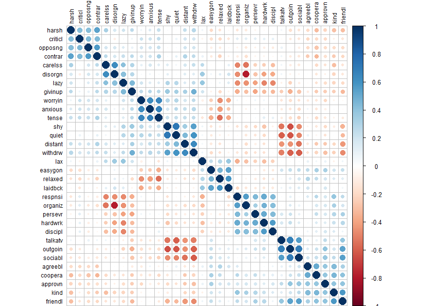
corrplot(cor(d), order = "hclust", tl.col='black', tl.cex=.75)

library(psych)
d.fa <- fa(d, rotate="none") # fa test with no rotation
names(d.fa) # to see what comes with the output d.fa
> names(d.fa)
 [1] "residual"      "dof"           "chi"           "nh"
 [5] "rms"           "EPVAL"         "crms"          "EBIC"
 [9] "ESABIC"        "fit"           "fit.off"       "sd"
[13] "factors"       "complexity"    "n.obs"         "objective"
[17] "criteria"      "STATISTIC"     "PVAL"          "Call"
[21] "null.model"    "null.dof"      "null.chisq"    "TLI"
[25] "RMSEA"         "BIC"           "SABIC"         "r.scores"
[29] "R2"            "valid"         "weights"       "rotation"
[33] "communality"   "communalities" "uniquenesses"  "values"
[37] "e.values"      "loadings"      "model"         "fm"
[41] "Structure"     "method"        "scores"        "R2.scores"
[45] "r"             "np.obs"        "fn"            "Vaccounted"
plot(d.fa$e.values, type='b')
d.fa$e.values

# 6 under eigenvalue 1
d.fa <- fa(d, nfactors=6, rotate="varimax")
d.fa.so <- fa.sort(d.fa)
d.fa.so

Factor Analysis using method =  minres
Call: fa(r = d, nfactors = 6, rotate = "varimax")
Standardized loadings (pattern matrix) based upon correlation matrix
          MR1   MR2   MR4   MR5   MR3   MR6   h2   u2 com
outgoin -0.82  0.10 -0.06  0.22  0.00  0.00 0.74 0.26 1.2
quiet    0.79 -0.16  0.18  0.17  0.02 -0.04 0.71 0.29 1.3
talkatv -0.75  0.06 -0.03  0.11  0.15  0.13 0.62 0.38 1.2
withdrw  0.74 -0.07  0.12 -0.10  0.25  0.14 0.67 0.33 1.4
sociabl -0.73 -0.07 -0.08  0.27 -0.06 -0.07 0.63 0.37 1.4
shy      0.71 -0.23  0.16  0.01 -0.07  0.01 0.59 0.41 1.4
distant  0.60  0.01  0.07 -0.12  0.27  0.16 0.48 0.52 1.7
discipl  0.06  0.69  0.04  0.07  0.03 -0.14 0.51 0.49 1.1
hardwrk -0.17  0.69  0.14  0.10  0.05 -0.16 0.56 0.44 1.4
lazy     0.17 -0.67  0.07  0.04  0.18  0.24 0.58 0.42 1.6
persevr -0.14  0.61  0.11  0.18  0.04 -0.09 0.44 0.56 1.4
respnsi -0.01  0.59  0.07  0.24  0.02 -0.41 0.58 0.42 2.2
givinup  0.35 -0.46  0.22 -0.09  0.17  0.15 0.44 0.56 3.1
lax      0.04 -0.38 -0.22  0.22  0.11  0.27 0.33 0.67 3.5
tense    0.16  0.03  0.77  0.01  0.26  0.07 0.69 0.31 1.3
worryin  0.17 -0.08  0.74  0.06  0.15  0.00 0.60 0.40 1.2
relaxed -0.02 -0.12 -0.69  0.34 -0.07  0.05 0.62 0.38 1.6
anxious  0.17 -0.02  0.69  0.15  0.21  0.13 0.59 0.41 1.5
laidbck -0.02 -0.18 -0.60  0.27  0.08  0.16 0.50 0.50 1.8
easygon -0.14 -0.16 -0.45  0.44  0.00  0.01 0.43 0.57 2.4
agreebl -0.02  0.04 -0.06  0.63 -0.19  0.10 0.45 0.55 1.3
kind    -0.11  0.20  0.04  0.62 -0.16 -0.23 0.53 0.47 1.8
coopera -0.10  0.16 -0.11  0.57 -0.29 -0.07 0.46 0.54 1.9
friendl -0.50  0.14  0.06  0.55 -0.15 -0.08 0.61 0.39 2.3
approvn -0.26  0.13 -0.12  0.50 -0.12 -0.03 0.37 0.63 2.0
contrar  0.05 -0.08  0.14 -0.15  0.72  0.13 0.59 0.41 1.3
opposng -0.01 -0.08  0.09 -0.13  0.65  0.07 0.46 0.54 1.2
harsh    0.08 -0.02  0.06 -0.23  0.62  0.18 0.48 0.52 1.5
criticl  0.08  0.11  0.15 -0.10  0.60 -0.13 0.43 0.57 1.4
disorgn  0.01 -0.36 -0.02  0.00  0.07  0.77 0.73 0.27 1.4
organiz -0.08  0.43  0.00  0.10  0.02 -0.71 0.71 0.29 1.7
carelss  0.05 -0.28  0.07 -0.06  0.21  0.65 0.55 0.45 1.7

                       MR1  MR2  MR4  MR5  MR3  MR6
SS loadings           4.50 3.19 2.97 2.55 2.31 2.16
Proportion Var        0.14 0.10 0.09 0.08 0.07 0.07
Cumulative Var        0.14 0.24 0.33 0.41 0.48 0.55
Proportion Explained  0.25 0.18 0.17 0.14 0.13 0.12
Cumulative Proportion 0.25 0.43 0.60 0.75 0.88 1.00

Mean item complexity =  1.7
Test of the hypothesis that 6 factors are sufficient.

The degrees of freedom for the null model are  496  and the objective function was  17.62 with Chi Square of  4009.54
The degrees of freedom for the model are 319  and the objective function was  2.48

The root mean square of the residuals (RMSR) is  0.03
The df corrected root mean square of the residuals is  0.04

The harmonic number of observations is  240 with the empirical chi square  229.67  with prob <  1
The total number of observations was  240  with Likelihood Chi Square =  553.98  with prob <  6.8e-15

Tucker Lewis Index of factoring reliability =  0.894
RMSEA index =  0.06  and the 90 % confidence intervals are  0.048 0.063
BIC =  -1194.35
Fit based upon off diagonal values = 0.99
Measures of factor score adequacy
                                                   MR1  MR2  MR4  MR5
Correlation of (regression) scores with factors   0.95 0.89 0.93 0.90
Multiple R square of scores with factors          0.91 0.80 0.86 0.81
Minimum correlation of possible factor scores     0.82 0.60 0.72 0.62
                                                   MR3  MR6
Correlation of (regression) scores with factors   0.89 0.88
Multiple R square of scores with factors          0.79 0.78
Minimum correlation of possible factor scores     0.58 0.56
outgoin -0.82  0.10 -0.06  0.22  0.00  0.00 0.74 0.26 1.2
quiet    0.79 -0.16  0.18  0.17  0.02 -0.04 0.71 0.29 1.3
talkatv -0.75  0.06 -0.03  0.11  0.15  0.13 0.62 0.38 1.2
withdrw  0.74 -0.07  0.12 -0.10  0.25  0.14 0.67 0.33 1.4
sociabl -0.73 -0.07 -0.08  0.27 -0.06 -0.07 0.63 0.37 1.4
shy      0.71 -0.23  0.16  0.01 -0.07  0.01 0.59 0.41 1.4
distant  0.60  0.01  0.07 -0.12  0.27  0.16 0.48 0.52 1.7
----
discipl  0.06  0.69  0.04  0.07  0.03 -0.14 0.51 0.49 1.1
hardwrk -0.17  0.69  0.14  0.10  0.05 -0.16 0.56 0.44 1.4
lazy     0.17 -0.67  0.07  0.04  0.18  0.24 0.58 0.42 1.6
persevr -0.14  0.61  0.11  0.18  0.04 -0.09 0.44 0.56 1.4
respnsi -0.01  0.59  0.07  0.24  0.02 -0.41 0.58 0.42 2.2
givinup  0.35 -0.46  0.22 -0.09  0.17  0.15 0.44 0.56 3.1
lax      0.04 -0.38 -0.22  0.22  0.11  0.27 0.33 0.67 3.5
----
tense    0.16  0.03  0.77  0.01  0.26  0.07 0.69 0.31 1.3
worryin  0.17 -0.08  0.74  0.06  0.15  0.00 0.60 0.40 1.2
relaxed -0.02 -0.12 -0.69  0.34 -0.07  0.05 0.62 0.38 1.6
anxious  0.17 -0.02  0.69  0.15  0.21  0.13 0.59 0.41 1.5
laidbck -0.02 -0.18 -0.60  0.27  0.08  0.16 0.50 0.50 1.8
easygon -0.14 -0.16 -0.45  0.44  0.00  0.01 0.43 0.57 2.4
----
agreebl -0.02  0.04 -0.06  0.63 -0.19  0.10 0.45 0.55 1.3
kind    -0.11  0.20  0.04  0.62 -0.16 -0.23 0.53 0.47 1.8
coopera -0.10  0.16 -0.11  0.57 -0.29 -0.07 0.46 0.54 1.9
friendl -0.50  0.14  0.06  0.55 -0.15 -0.08 0.61 0.39 2.3
approvn -0.26  0.13 -0.12  0.50 -0.12 -0.03 0.37 0.63 2.0
----
contrar  0.05 -0.08  0.14 -0.15  0.72  0.13 0.59 0.41 1.3
opposng -0.01 -0.08  0.09 -0.13  0.65  0.07 0.46 0.54 1.2
harsh    0.08 -0.02  0.06 -0.23  0.62  0.18 0.48 0.52 1.5
criticl  0.08  0.11  0.15 -0.10  0.60 -0.13 0.43 0.57 1.4
----
disorgn  0.01 -0.36 -0.02  0.00  0.07  0.77 0.73 0.27 1.4
organiz -0.08  0.43  0.00  0.10  0.02 -0.71 0.71 0.29 1.7
carelss  0.05 -0.28  0.07 -0.06  0.21  0.65 0.55 0.45 1.7
----
communality
> fa.sort(data.frame(d.fa.so$communality))
        d.fa.so.communality order
outgoin           0.7376260     1
disorgn           0.7329193    30
organiz           0.7136615    31
quiet             0.7107357     2
tense             0.6925168    15
withdrw           0.6650390     4
sociabl           0.6302538     5
talkatv           0.6221579     3
relaxed           0.6166856    17
friendl           0.6063722    24
worryin           0.6046637    16
contrar           0.5949600    26
anxious           0.5893186    18
shy               0.5859167     6
lazy              0.5771937    10
respnsi           0.5750101    12
hardwrk           0.5585236     9
carelss           0.5523099    32
kind              0.5251513    22
discipl           0.5096792     8
laidbck           0.4980387    19
harsh             0.4791709    28
distant           0.4785914     7
coopera           0.4574619    23
opposng           0.4572599    27
agreebl           0.4508557    21
persevr           0.4442142    11
givinup           0.4409678    13
easygon           0.4340117    20
criticl           0.4333566    29
approvn           0.3705982    25
lax               0.3295470    14
>
eigenvalues
위의 아웃풋에서 (d.fa.so)
SS loadings (eigenvalue 라고 부른다)
                       MR1  MR2  MR4  MR5  MR3  MR6
SS loadings           4.50 3.19 2.97 2.55 2.31 2.16
Proportion Var        0.14 0.10 0.09 0.08 0.07 0.07
Cumulative Var        0.14 0.24 0.33 0.41 0.48 0.55
Proportion Explained  0.25 0.18 0.17 0.14 0.13 0.12
Cumulative Proportion 0.25 0.43 0.60 0.75 0.88 1.00

SS loadings = eigenvalues for each factor (MR1, . . . )
SS loadings 4.50
# SS total = 각 변인들의 분산을 (variation) 1 로 보았을 때 SS loading 값을 구한 것이므로
# SS total 값은 각 변인들의 숫자만큼이 된다. 이 경우는 총 32개 문항이 존재하므로 32가 SS total
ss.tot = 32
SS total 32 (성격변인 들의 SS값을 모두 더한 값 즉, 각 변인의 SS값을 구하여 이를 더한 값)
$\frac {4.5}{32} = 0.14$
Proportion Var 0.14
eigenvalues for factor 1
| SS loadings eigenvalue | 4.50 | 3.19 | 2.97 | 2.55 | 2.31 | 2.16 |
| $\frac {4.5}{32}$ | $\frac {3.19}{32}$ | $\frac {2.97}{32}$ | $\frac {2.55}{32}$ | $\frac {2.31}{32}$ | $\frac {2.16}{32}$ | |
| Proportion Var | 0.14 | 0.10 | 0.09 | 0.08 | 0.07 | 0.07 |
| Cumulative Var | 0.14 | 0.24 | 0.33 | 0.41 | 0.48 | 0.55 |
아래는 loading값 중 첫번 째 팩터의 합을 (eigenvalue) 체크하는 방법
d.fa.so$loadings
d.fa.so.loadings.f1 <- d.fa.so$loadings[,1]
ev_fa1 <- sum(data.frame(d.fa.so.loadings.f1)^2)
# this value should be matched with SS loadings for MR1
ev_fa1
[1] 4.500258
> (4.50+3.19+2.97+2.55+2.31+2.16)/32
[1] 0.5525

> or
sum(d.fa.so.loadings^2)/ss.tot
specific variance
1 - communality
Uniqueness
data.frame(d.fa.so$uniquenesses)
        d.fa.so.uniquenesses
outgoin           0.2623740
quiet             0.2892643
talkatv           0.3778421
withdrw           0.3349610
sociabl           0.3697462
shy               0.4140833
distant           0.5214086
discipl           0.4903208
hardwrk           0.4414764
lazy              0.4228063
persevr           0.5557858
respnsi           0.4249899
givinup           0.5590322
lax               0.6704530
tense             0.3074832
worryin           0.3953363
relaxed           0.3833144
anxious           0.4106814
laidbck           0.5019613
easygon           0.5659883
agreebl           0.5491443
kind              0.4748487
coopera           0.5425381
friendl           0.3936278
approvn           0.6294018
contrar           0.4050400
opposng           0.5427401
harsh             0.5208291
criticl           0.5666434
disorgn           0.2670807
organiz           0.2863385
carelss           0.4476901
>
uniqueness for variable 1 (v1)
> d.fa.so.loadings.v1 <- d.fa.so$loadings[1,]
> d.fa.so.communality.v1 <- sum(d.fa.so.loadings.v1^2)
> d.fa.so.uniqeness.v1 <- 1 - d.fa.so.communality.v1
> d.fa.so.communality.v1
[1] 0.737626
> d.fa.so.uniqeness.v1
[1] 0.262374
>
d.fa.so.communality.v1 = [1] 0.737626 = 0.74
d.fa.so.uniqeness.v1 = [1] 0.262374 = 0.26
plotting
intronductory
load12 <- d.fa.so$loadings[,1:2] # for factor 1 and 2
plot(load12, type='n')
text(load12, labels=names(d.fa.so.loadings.f1), cex=.7)
load23 <- d.fa.so$loadings[,2:3] # for factor 1 and 2
plot(load23, type='n')
text(load23, labels=names(d.fa.so.loadings.f1), cex=.7)
load123 <- d.fa.so$loadings[,1:3] # for factor 1 and 2
plot(load123, type='n')
text(load123, labels=names(d.fa.so.loadings.f1), cex=.7)
E.g., 4
medfactor.txt
medical data: 11 variables (exam items: such as lung, heart, liver, etc.)
n = 128 participants
mission: the items could be factored into how many and how?
med.dat <- read.table("http://commres.net/wiki/_media/r/medfactor.txt", header = T)
head(med.dat)

  lung muscle liver skeleton kidneys heart step stamina stretch blow urine
1   20     16    52       10      24    23   19      20      23   29    67
2   24     16    52        7      27    16   16      15      31   33    59
3   19     21    57       18      22    23   16      19      42   40    61
4   24     21    62       12      31    25   17      17      36   36    77
5   29     18    62       14      26    27   15      20      33   29    88
6   18     19    51       15      29    23   19      20      50   37    54
med.factor = fa(med.dat, rotate='none')
names(med.factor)
# med.factor$e.values = eigenvalues
# find how many items are over the value 1.
med.factor$e.values
 [1] 3.3791814 1.4827707 1.2506302 0.9804771 0.7688022 0.7330511 0.6403994
 [8] 0.6221934 0.5283718 0.3519301 0.2621928
plot(med.factor$e.values, type = "b")
the eigenvalues of 3-4 factors are over 1.
med.fa.varimax <- fa(med.dat, nfactors = 3, rotate = "varimax")
med.fa.varimax
Factor Analysis using method =  minres
Call: fa(r = med.dat, nfactors = 3, rotate = "varimax")
Standardized loadings (pattern matrix) based upon correlation matrix
           MR1   MR3   MR2   h2     u2 com
lung      0.56  0.13  0.16 0.36 0.6401 1.3
muscle    0.17 -0.05  0.42 0.21 0.7949 1.4
liver     0.83  0.11  0.12 0.71 0.2869 1.1
skeleton  0.13  0.26  0.96 1.00 0.0021 1.2
kidneys   0.54  0.26  0.01 0.36 0.6351 1.4
heart     0.44  0.01  0.19 0.23 0.7715 1.4
step      0.42  0.42  0.12 0.37 0.6284 2.2
stamina   0.11  0.45  0.18 0.24 0.7555 1.4
stretch   0.21  0.55  0.28 0.43 0.5734 1.8
blow      0.23  0.66 -0.01 0.49 0.5128 1.2
urine    -0.03  0.46 -0.11 0.22 0.7789 1.1

                       MR1  MR3  MR2
SS loadings           1.82 1.49 1.30
Proportion Var        0.17 0.14 0.12
Cumulative Var        0.17 0.30 0.42
Proportion Explained  0.39 0.32 0.28
Cumulative Proportion 0.39 0.72 1.00

Mean item complexity =  1.4
Test of the hypothesis that 3 factors are sufficient.

The degrees of freedom for the null model are  55  and the objective function was  2.7 with Chi Square of  330.64
The degrees of freedom for the model are 25  and the objective function was  0.41

The root mean square of the residuals (RMSR) is  0.05
The df corrected root mean square of the residuals is  0.07

The harmonic number of observations is  128 with the empirical chi square  35  with prob <  0.088
The total number of observations was  128  with Likelihood Chi Square =  49.59  with prob <  0.0024

Tucker Lewis Index of factoring reliability =  0.8
RMSEA index =  0.093  and the 90 % confidence intervals are  0.051 0.124
BIC =  -71.71
Fit based upon off diagonal values = 0.96
Measures of factor score adequacy
                                                   MR1  MR3  MR2
Correlation of (regression) scores with factors   0.88 0.81 0.99
Multiple R square of scores with factors          0.77 0.66 0.99
Minimum correlation of possible factor scores     0.55 0.32 0.98
factor loadings for each factor (total 3) and h2 (communality) and u2 (uniqueness or specific variance), and com (?).
> names(med.fa.varimax)
 [1] "residual"      "dof"           "chi"           "nh"
 [5] "rms"           "EPVAL"         "crms"          "EBIC"
 [9] "ESABIC"        "fit"           "fit.off"       "sd"
[13] "factors"       "complexity"    "n.obs"         "objective"
[17] "criteria"      "STATISTIC"     "PVAL"          "Call"
[21] "null.model"    "null.dof"      "null.chisq"    "TLI"
[25] "RMSEA"         "BIC"           "SABIC"         "r.scores"
[29] "R2"            "valid"         "score.cor"     "weights"
[33] "rotation"      "communality"   "communalities" "uniquenesses"
[37] "values"        "e.values"      "loadings"      "model"
[41] "fm"            "rot.mat"       "Structure"     "method"
[45] "scores"        "R2.scores"     "r"             "np.obs"
[49] "fn"            "Vaccounted"
- loadings = factor loadings
- e.values = estimated eigenvalues according to the number of factors
- communality = communality
- uniqueness = spec. variance
med.fa.varimax$loadings

Loadings:
         MR1    MR3    MR2
lung      0.563  0.129  0.163
muscle    0.173         0.416
liver     0.828  0.109  0.123
skeleton  0.127  0.255  0.957
kidneys   0.544  0.263
heart     0.437         0.192
step      0.421  0.425  0.120
stamina   0.108  0.449  0.178
stretch   0.206  0.554  0.278
blow      0.233  0.658
urine            0.455 -0.113

                 MR1   MR3   MR2
SS loadings    1.822 1.493 1.305
Proportion Var 0.166 0.136 0.119
Cumulative Var 0.166 0.301 0.420
> fa.sort(med.fa.varimax)
Factor Analysis using method =  minres
Call: fa(r = med.dat, nfactors = 3, rotate = "varimax")
Standardized loadings (pattern matrix) based upon correlation matrix
           MR1   MR3   MR2   h2     u2 com
liver     0.83  0.11  0.12 0.71 0.2869 1.1
lung      0.56  0.13  0.16 0.36 0.6401 1.3
kidneys   0.54  0.26  0.01 0.36 0.6351 1.4
heart     0.44  0.01  0.19 0.23 0.7715 1.4
blow      0.23  0.66 -0.01 0.49 0.5128 1.2
stretch   0.21  0.55  0.28 0.43 0.5734 1.8
urine    -0.03  0.46 -0.11 0.22 0.7789 1.1
stamina   0.11  0.45  0.18 0.24 0.7555 1.4
step      0.42  0.42  0.12 0.37 0.6284 2.2
skeleton  0.13  0.26  0.96 1.00 0.0021 1.2
muscle    0.17 -0.05  0.42 0.21 0.7949 1.4

                       MR1  MR3  MR2
SS loadings           1.82 1.49 1.30
Proportion Var        0.17 0.14 0.12
Cumulative Var        0.17 0.30 0.42
Proportion Explained  0.39 0.32 0.28
Cumulative Proportion 0.39 0.72 1.00

Mean item complexity =  1.4
Test of the hypothesis that 3 factors are sufficient.

The degrees of freedom for the null model are  55  and the objective function was  2.7 with Chi Square of  330.64
The degrees of freedom for the model are 25  and the objective function was  0.41

The root mean square of the residuals (RMSR) is  0.05
The df corrected root mean square of the residuals is  0.07

The harmonic number of observations is  128 with the empirical chi square  35  with prob <  0.088
The total number of observations was  128  with Likelihood Chi Square =  49.59  with prob <  0.0024

Tucker Lewis Index of factoring reliability =  0.8
RMSEA index =  0.093  and the 90 % confidence intervals are  0.051 0.124
BIC =  -71.71
Fit based upon off diagonal values = 0.96
Measures of factor score adequacy
                                                   MR1  MR3  MR2
Correlation of (regression) scores with factors   0.88 0.81 0.99
Multiple R square of scores with factors          0.77 0.66 0.99
Minimum correlation of possible factor scores     0.55 0.32 0.98
>
sorted values in factor loadings will help.
liver     0.83  0.11  0.12 0.71 0.2869 1.1
lung      0.56  0.13  0.16 0.36 0.6401 1.3
kidneys   0.54  0.26  0.01 0.36 0.6351 1.4
heart     0.44  0.01  0.19 0.23 0.7715 1.4

blow            0.66 -0.01 0.49 0.5128 1.2
stretch         0.55  0.28 0.43 0.5734 1.8
urine           0.46 -0.11 0.22 0.7789 1.1
stamina         0.45  0.18 0.24 0.7555 1.4
step            0.42  0.12 0.37 0.6284 2.2

skeleton              0.96 1.00 0.0021 1.2
muscle                0.42 0.21 0.7949 1.4
liver, lung, kidneys, heart scores are on F1
blow, stretch, urine, stamina, step are on F2
skeleton, muscle are on F3
F1 could be named as biomedical information
F2 could be performance
F3 could be strength
Now we could state that the tests are composed of three dimensions: biomedical info, performance, and strength.
excersize
| Variable | Position | Label |
|---|---|---|
| stat_cry | 1 | Statiscs makes me cry |
| afraid_spss | 2 | My friends will think I'm stupid for not being able to cope with SPSS |
| sd_excite | 3 | Standard deviations excite me |
| nmare_pearson | 4 | I dream that Pearson is attacking me with correlation coefficients |
| du_stat | 5 | I don't understand statistics |
| lexp_comp | 6 | I have little experience of computers |
| comp_hate | 7 | All computers hate me |
| good_math | 8 | I have never been good at mathematics |
| frs_better_stat | 9 | My friends are better at statistics than me |
| com_for_games | 10 | Computers are useful only for playing games |
| bad_math | 11 | I did badly at mathematics at school |
| spss_no_help | 12 | People try to tell you that SPSS makes statistics easier to understand but it doesn't |
| damaging_comp | 13 | I worry that I will cause irreparable damage because of my incompetenece with computers |
| comp_alive | 14 | Computers have minds of their own and deliberately go wrong whenever I use them |
| comp_getme | 15 | Computers are out to get me |
| weep_ct | 16 | I weep openly at the mention of central tendency |
| slip_coma | 17 | I slip into a coma whenever I see an equation |
| spss_crash | 18 | SPSS always crashes when I try to use it |
| eb_looks | 19 | Everybody looks at me when I use SPSS |
| no_sleep_ev | 20 | I can't sleep for thoughts of eigen vectors |
| nm_normdist | 21 | I wake up under my duvet thinking that I am trapped under a normal distribtion |
| frs_better_spss | 22 | My friends are better at SPSS than I am |
| stat_nerd | 23 | If I'm good at statistics my friends will think I'm a nerd |
saq <- read.csv("http://commres.net/wiki/_media/r/saq.csv", header = T)
head(saq)
see SAQ dataset
e.g., 5
e.g. secu com finance 2007 example
Sys.setlocale("LC_ALL","Korean")
secu_com_finance_2007 <- read.csv("http://commres.net/wiki/_media/r/secu_com_finance_2007.csv")
secu_com_finance_2007

# V1 : 총자본순이익율
# V2 : 자기자본순이익율
# V3 : 자기자본비율
# V4 : 부채비율
# V5 : 자기자본회전율

# 표준화 변환 (standardization)
secu_com_finance_2007 <- transform(secu_com_finance_2007,
    V1_s = scale(V1),
    V2_s = scale(V2),
    V3_s = scale(V3),
    V4_s = scale(V4),
    V5_s = scale(V5))

# 부채비율(V4_s)을 방향(max(V4_s)-V4_s) 변환
secu_com_finance_2007 <- transform(secu_com_finance_2007, V4_s2 = max(V4_s) - V4_s)

# variable selection
secu_com_finance_2007_2 <- secu_com_finance_2007[,c("company", "V1_s", "V2_s", "V3_s", "V4_s2", "V5_s")]

# Correlation analysis
cor(secu_com_finance_2007_2[,-1])

round(cor(secu_com_finance_2007_2[,-1]), digits=3) # 반올림

# Scatter plot matrix
plot(secu_com_finance_2007_2[,-1])

# Scree Plot
plot(prcomp(secu_com_finance_2007_2[,c(2:6)]), type="l", sub = "Scree Plot")
# 요인분석(maximum likelihood factor analysis)
# rotation = "varimax"
secu_factanal <- factanal(secu_com_finance_2007_2[,2:6],
    factors = 2,
    rotation = "varimax", # "varimax", "promax", "none"
    scores="regression") # "regression", "Bartlett"
print(secu_factanal)
print(secu_factanal$loadings, cutoff=0) # display every loadings

# factor scores plotting
secu_factanal$scores

plot(secu_factanal$scores, main="Biplot of the first 2 factors")

# 관측치별 이름 매핑(rownames mapping)
text(secu_factanal$scores[,1], secu_factanal$scores[,2],
   labels = secu_com_finance_2007$company,
   cex = 0.7, pos = 3, col = "blue")

# factor loadings plotting
points(secu_factanal$loadings, pch=19, col = "red")


text(secu_factanal$loadings[,1], secu_factanal$loadings[,2],
   labels = rownames(secu_factanal$loadings),
   cex = 0.8, pos = 3, col = "red")

# plotting lines between (0,0) and (factor loadings by Var.)
segments(0,0,secu_factanal$loadings[1,1], secu_factanal$loadings[1,2])
segments(0,0,secu_factanal$loadings[2,1], secu_factanal$loadings[2,2])
segments(0,0,secu_factanal$loadings[3,1], secu_factanal$loadings[3,2])
segments(0,0,secu_factanal$loadings[4,1], secu_factanal$loadings[4,2])
segments(0,0,secu_factanal$loadings[5,1], secu_factanal$loadings[5,2])
e.g
etc.
Reference
Lecture Note from databaser
https://stats.oarc.ucla.edu/spss/seminars/introduction-to-factor-analysis/a-practical-introduction-to-factor-analysis/
https://advstats.psychstat.org/book/factor/efa.php
see exploratory factor analysis ::