This is an old revision of the document!
Table of Contents
Multiple Regression with Two Predictor Variables
data file: mlt06.sav from http://www.psychstat.missouristate.edu/multibook/mlt06.htm
- Y1 - A measure of success in graduate school.
- X1 - A measure of intellectual ability.
- X2 - A measure of “work ethic.”
- X3 - A second measure of intellectual ability.
- X4 - A measure of spatial ability.
- Y2 - Score on a major review paper.
Analyze
 Descriptive statistics
  Descriptives
   모든 변수를 Variable(s)로 이동
    OK 누르기
Descriptive Statistics
				N	Minimum	Maximum	Mean	Std. Deviation
sucess in graduate school	20	125	230	169.45	24.517
score on a major review paper	20	105	135	120.50	8.918
intellectual ability I		20	11	64	37.05	14.891
work ethic			20	11	56	29.10	14.056
intellectual ability II		20	17	79	49.35	18.622
spatial ability			20	11	56	32.50	13.004
Valid N (listwise)		20
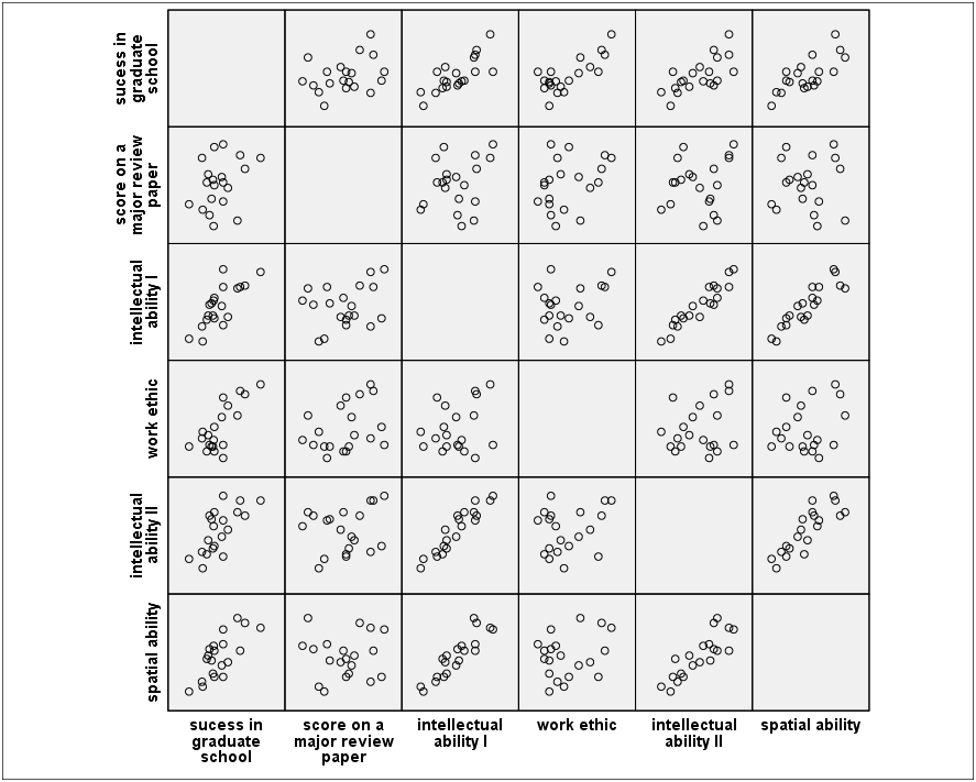
Correlation matrix 검사
Analyze
 Correlate
  Bivariate
   모든 변수를 Variable(s)로 이동
Correlations
				y1	y2	x1	x2	x3	x4
y1	Pearson Correlation	1	.310	.764**	.769**	.687**	.736**
	Sig. (2-tailed)		.184	.000	.000	.001	.000
	N			20	20	20	20	20	20
y2	Pearson Correlation	.310	1	.251	.334	.168	.018
	Sig. (2-tailed)		.184		.286	.150	.479	.939
	N			20	20	20	20	20	20
x1	Pearson Correlation	.764**	.251	1	.255	.940**	.904**
	Sig. (2-tailed)		.000	.286		.278	.000	.000
	N			20	20	20	20	20	20
x2	Pearson Correlation	.769**	.334	.255	1	.243	.266
	Sig. (2-tailed)		.000	.150	.278		.302	.257
	N			20	20	20	20	20	20
x3	Pearson Correlation	.687**	.168	.940**	.243	1	.847**
	Sig. (2-tailed)		.001	.479	.000	.302		.000
	N			20	20	20	20	20	20
x4	Pearson Correlation	.736**	.018	.904**	.266	.847**	1
	Sig. (2-tailed)		.000	.939	.000	.257	.000
	N			20	20	20	20	20	20
** Correlation is significant at the 0.01 level (2-tailed).
Regression
Analyze
 Regression
  Linear
   Dependent: 	y1 (success in graduate school)
   Independent:	x1 (intell. ability)
		x2 (work ethic)
   Click Statistics (오른쪽 상단 버튼)
    Choose
     Estimates (under Regression Coefficients)
     Model fit
     R squared change
     Descriptives
     Part and partial correlations
     Collinearity diagnostics
Model Summaryb
							Change Statistics
Model	R	R	Adjusted	Std. Error	R  	F 	df1	df2	Sig. F
		Square	R Square	of the 		Square	Change			Change
					Estimate	Change
1	.968a	.936	.929		6.541		.936	124.979	2	17	.000
a Predictors: (Constant), work ethic, intellectual ability I
b Dependent Variable: success in graduate school
ANOVAa
Model			Sum of Squares	df	Mean Square	F		Sig.
1	Regression	10693.657	2	5346.828	124.979		.000b
	Residual	727.293		17	42.782
	Total		11420.950	19
a Dependent Variable: sucess in graduate school
b Predictors: (Constant), work ethic, intellectual ability I
Coefficientsa
Model		Unstandardized 	Standardized 		Correlations		Collinearity
		Coefficients	Coefficients					Statistics
		-------------	-----	------------	--------------------	---------	----
		B	Std. 	Beta	t	Sig.	Zero	Partial	Part	Tolerance	VIF
			Error					-order
1 (Constant)	101.222	4.587		22.065	.000
  x1		1.000	.104	.608	9.600	.000	.764	.919	.588	.935		1.070
  x3		1.071	.110	.614	9.699	.000	.769	.920	.594	.935		1.070
a Dependent Variable: success in graduate school
x1  intellectual ability I
x3  work ethic
from the above output:
| x | zero-order cor | part cor | squared zero-order cor | squared part cor | shared square cor |
| x1 | .764 | .588 | 0.583696 | 0.345744 | 0.237952 |
| x2 | .769 | .594 | 0.591361 | 0.352836 | 0.238525 |
note that the values of two raws at the last column are similar. The portion is the shared effects from both x1 and x2.
$$ \hat{Y_{i}} = 101.222 + 1.000X1_{i} + 1.071X2_{i} $$
$$ \hat{Y_{i}} = 101.222 + 1.000 \ \text{intell. ability}_{i} + 1.071 \ \text{work ethic}_{i} $$
E.g. 2
?state.x77
US State Facts and Figures
Description
Data sets related to the 50 states of the United States of America.
Usage
state.abb
state.area
state.center
state.division
state.name
state.region
state.x77
Details
R currently contains the following “state” data sets. Note that all data are arranged according to alphabetical order of the state names.
state.abb:
character vector of 2-letter abbreviations for the state names.
state.area:
numeric vector of state areas (in square miles).
state.center:
list with components named x and y giving the approximate geographic center of each state in negative longitude and latitude. Alaska and Hawaii are placed just off the West Coast.
state.division:
factor giving state divisions (New England, Middle Atlantic, South Atlantic, East South Central, West South Central, East North Central, West North Central, Mountain, and Pacific).
state.name:
character vector giving the full state names.
state.region:
factor giving the region (Northeast, South, North Central, West) that each state belongs to.
state.x77:
matrix with 50 rows and 8 columns giving the following statistics in the respective columns.
Population:
population estimate as of July 1, 1975
Income:
per capita income (1974)
Illiteracy:
illiteracy (1970, percent of population)
Life Exp:
life expectancy in years (1969–71)
Murder:
murder and non-negligent manslaughter rate per 100,000 population (1976)
HS Grad:
percent high-school graduates (1970)
Frost:
mean number of days with minimum temperature below freezing (1931–1960) in capital or large city
Area:
land area in square miles
Source
U.S. Department of Commerce, Bureau of the Census (1977) Statistical Abstract of the United States.
U.S. Department of Commerce, Bureau of the Census (1977) County and City Data Book.
References
Becker, R. A., Chambers, J. M. and Wilks, A. R. (1988) The New S Language. Wadsworth & Brooks/Cole.
> state.x77                            # output not shown
> str(state.x77)                       # clearly not a data frame! (it's a matrix)
> st = as.data.frame(state.x77)        # so we'll make it one
> str(st)
'data.frame':   50 obs. of  8 variables:
 $ Population: num   3615   365  2212  2110 21198 ...
 $ Income    : num  3624 6315 4530 3378 5114 ...
 $ Illiteracy: num  2.1 1.5 1.8 1.9 1.1 0.7 1.1 0.9 1.3 2 ...
 $ Life Exp  : num  69.0 69.3 70.5 70.7 71.7 ...
 $ Murder    : num  15.1 11.3 7.8 10.1 10.3 6.8 3.1 6.2 10.7 13.9 ...
 $ HS Grad   : num  41.3 66.7 58.1 39.9 62.6 63.9 56 54.6 52.6 40.6 ...
 $ Frost     : num  20 152 15 65 20 166 139 103 11 60 ...
 $ Area      : num   50708 566432 113417  51945 156361 ...
> colnames(st)[4] = "Life.Exp"                   # no spaces in variable names, please
> colnames(st)[6] = "HS.Grad"                    # ditto
> st$Density = st$Population * 1000 / st$Area    # create a new column in st
> summary(st)
   Population        Income       Illiteracy       Life.Exp         Murder
 Min.   :  365   Min.   :3098   Min.   :0.500   Min.   :67.96   Min.   : 1.400
 1st Qu.: 1080   1st Qu.:3993   1st Qu.:0.625   1st Qu.:70.12   1st Qu.: 4.350
 Median : 2838   Median :4519   Median :0.950   Median :70.67   Median : 6.850
 Mean   : 4246   Mean   :4436   Mean   :1.170   Mean   :70.88   Mean   : 7.378
 3rd Qu.: 4968   3rd Qu.:4814   3rd Qu.:1.575   3rd Qu.:71.89   3rd Qu.:10.675
 Max.   :21198   Max.   :6315   Max.   :2.800   Max.   :73.60   Max.   :15.100
    HS.Grad          Frost             Area           Density
 Min.   :37.80   Min.   :  0.00   Min.   :  1049   Min.   :  0.6444
 1st Qu.:48.05   1st Qu.: 66.25   1st Qu.: 36985   1st Qu.: 25.3352
 Median :53.25   Median :114.50   Median : 54277   Median : 73.0154
 Mean   :53.11   Mean   :104.46   Mean   : 70736   Mean   :149.2245
 3rd Qu.:59.15   3rd Qu.:139.75   3rd Qu.: 81162   3rd Qu.:144.2828
 Max.   :67.30   Max.   :188.00   Max.   :566432   Max.   :975.0033
> cor(st)                              # correlation matrix (not shown, yet)
> round(cor(st), 3)                    # rounding makes it easier to look at
           Population Income Illiteracy Life.Exp Murder HS.Grad  Frost   Area Density
Population      1.000  0.208      0.108   -0.068  0.344  -0.098 -0.332  0.023   0.246
Income          0.208  1.000     -0.437    0.340 -0.230   0.620  0.226  0.363   0.330
Illiteracy      0.108 -0.437      1.000   -0.588  0.703  -0.657 -0.672  0.077   0.009
Life.Exp       -0.068  0.340     -0.588    1.000 -0.781   0.582  0.262 -0.107   0.091
Murder          0.344 -0.230      0.703   -0.781  1.000  -0.488 -0.539  0.228  -0.185
HS.Grad        -0.098  0.620     -0.657    0.582 -0.488   1.000  0.367  0.334  -0.088
Frost          -0.332  0.226     -0.672    0.262 -0.539   0.367  1.000  0.059   0.002
Area            0.023  0.363      0.077   -0.107  0.228   0.334  0.059  1.000  -0.341
Density         0.246  0.330      0.009    0.091 -0.185  -0.088  0.002 -0.341   1.000
>
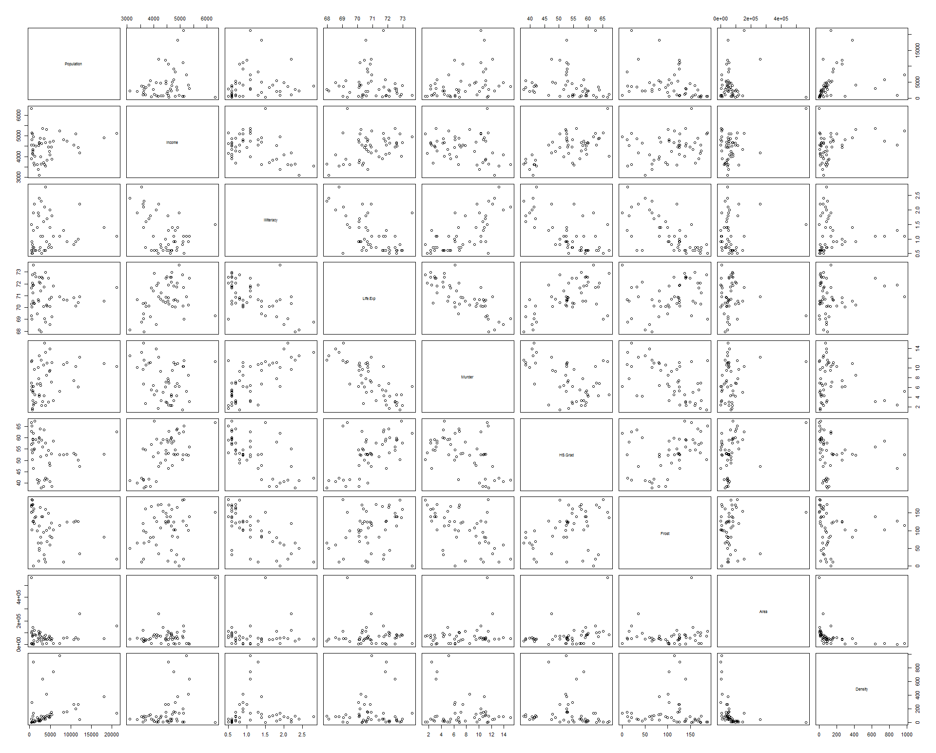
> pairs(st) # scatterplot matrix; plot(st) does the same thing
> ### model1 = lm(Life.Exp ~ Population + Income + Illiteracy + Murder +
+ ###                        HS.Grad + Frost + Area + Density, data=st)
> ### This is what we're going to accomplish, but more economically, by
> ### simply placing a dot after the tilde, which means "everything else."
> model1 = lm(Life.Exp ~ ., data=st)
> summary(model1)

Call:
lm(formula = Life.Exp ~ ., data = st)

Residuals:
     Min       1Q   Median       3Q      Max
-1.47514 -0.45887 -0.06352  0.59362  1.21823

Coefficients:
              Estimate Std. Error t value Pr(>|t|)
(Intercept)  6.995e+01  1.843e+00  37.956  < 2e-16 ***
Population   6.480e-05  3.001e-05   2.159   0.0367 *
Income       2.701e-04  3.087e-04   0.875   0.3867
Illiteracy   3.029e-01  4.024e-01   0.753   0.4559
Murder      -3.286e-01  4.941e-02  -6.652 5.12e-08 ***
HS.Grad      4.291e-02  2.332e-02   1.840   0.0730 .
Frost       -4.580e-03  3.189e-03  -1.436   0.1585
Area        -1.558e-06  1.914e-06  -0.814   0.4205
Density     -1.105e-03  7.312e-04  -1.511   0.1385
---
Signif. codes:  0 ‘***’ 0.001 ‘**’ 0.01 ‘*’ 0.05 ‘.’ 0.1 ‘ ’ 1

Residual standard error: 0.7337 on 41 degrees of freedom
Multiple R-squared:  0.7501,	Adjusted R-squared:  0.7013
F-statistic: 15.38 on 8 and 41 DF,  p-value: 3.787e-10
> summary.aov(model1)
            Df Sum Sq Mean Sq F value   Pr(>F)
Population   1  0.409   0.409   0.760  0.38849
Income       1 11.595  11.595  21.541 3.53e-05 ***
Illiteracy   1 19.421  19.421  36.081 4.23e-07 ***
Murder       1 27.429  27.429  50.959 1.05e-08 ***
HS.Grad      1  4.099   4.099   7.615  0.00861 **
Frost        1  2.049   2.049   3.806  0.05792 .
Area         1  0.001   0.001   0.002  0.96438
Density      1  1.229   1.229   2.283  0.13847
Residuals   41 22.068   0.538
---
Signif. codes:  0 ‘***’ 0.001 ‘**’ 0.01 ‘*’ 0.05 ‘.’ 0.1 ‘ ’ 1
>
Model fitting
> model2 = update(model1, .~. -Area)
> summary(model2)

Call:
lm(formula = Life.Exp ~ Population + Income + Illiteracy + Murder +
    HS.Grad + Frost + Density, data = st)

Residuals:
     Min       1Q   Median       3Q      Max
-1.50252 -0.40471 -0.06079  0.58682  1.43862

Coefficients:
              Estimate Std. Error t value Pr(>|t|)
(Intercept)  7.094e+01  1.378e+00  51.488  < 2e-16 ***
Population   6.249e-05  2.976e-05   2.100   0.0418 *
Income       1.485e-04  2.690e-04   0.552   0.5840
Illiteracy   1.452e-01  3.512e-01   0.413   0.6814
Murder      -3.319e-01  4.904e-02  -6.768 3.12e-08 ***
HS.Grad      3.746e-02  2.225e-02   1.684   0.0996 .
Frost       -5.533e-03  2.955e-03  -1.873   0.0681 .
Density     -7.995e-04  6.251e-04  -1.279   0.2079
---
Signif. codes:  0 ‘***’ 0.001 ‘**’ 0.01 ‘*’ 0.05 ‘.’ 0.1 ‘ ’ 1

Residual standard error: 0.7307 on 42 degrees of freedom
Multiple R-squared:  0.746,	Adjusted R-squared:  0.7037
F-statistic: 17.63 on 7 and 42 DF,  p-value: 1.173e-10
> anova(model2, model1)
Analysis of Variance Table

Model 1: Life.Exp ~ Population + Income + Illiteracy + Murder + HS.Grad +
    Frost + Density
Model 2: Life.Exp ~ Population + Income + Illiteracy + Murder + HS.Grad +
    Frost + Area + Density
  Res.Df    RSS Df Sum of Sq      F Pr(>F)
1     42 22.425
2     41 22.068  1   0.35639 0.6621 0.4205
> model3 = update(model2, .~. -Illiteracy)
> summary(model3)


Call:
lm(formula = Life.Exp ~ Population + Income + Murder + HS.Grad +
    Frost + Density, data = st)

Residuals:
     Min       1Q   Median       3Q      Max
-1.49555 -0.41246 -0.05336  0.58399  1.50535

Coefficients:
              Estimate Std. Error t value Pr(>|t|)
(Intercept)  7.131e+01  1.042e+00  68.420  < 2e-16 ***
Population   5.811e-05  2.753e-05   2.110   0.0407 *
Income       1.324e-04  2.636e-04   0.502   0.6181
Murder      -3.208e-01  4.054e-02  -7.912 6.32e-10 ***
HS.Grad      3.499e-02  2.122e-02   1.649   0.1065
Frost       -6.191e-03  2.465e-03  -2.512   0.0158 *
Density     -7.324e-04  5.978e-04  -1.225   0.2272
---
Signif. codes:  0 ‘***’ 0.001 ‘**’ 0.01 ‘*’ 0.05 ‘.’ 0.1 ‘ ’ 1

Residual standard error: 0.7236 on 43 degrees of freedom
Multiple R-squared:  0.745,	Adjusted R-squared:  0.7094
F-statistic: 20.94 on 6 and 43 DF,  p-value: 2.632e-11

>
> model4 = update(model3, .~. -Income)
> summary(model4)

Call:
lm(formula = Life.Exp ~ Population + Murder + HS.Grad + Frost +
    Density, data = st)

Residuals:
     Min       1Q   Median       3Q      Max
-1.56877 -0.40951 -0.04554  0.57362  1.54752

Coefficients:
              Estimate Std. Error t value Pr(>|t|)
(Intercept)  7.142e+01  1.011e+00  70.665  < 2e-16 ***
Population   6.083e-05  2.676e-05   2.273  0.02796 *
Murder      -3.160e-01  3.910e-02  -8.083 3.07e-10 ***
HS.Grad      4.233e-02  1.525e-02   2.776  0.00805 **
Frost       -5.999e-03  2.414e-03  -2.485  0.01682 *
Density     -5.864e-04  5.178e-04  -1.132  0.26360
---
Signif. codes:  0 ‘***’ 0.001 ‘**’ 0.01 ‘*’ 0.05 ‘.’ 0.1 ‘ ’ 1

Residual standard error: 0.7174 on 44 degrees of freedom
Multiple R-squared:  0.7435,	Adjusted R-squared:  0.7144
F-statistic: 25.51 on 5 and 44 DF,  p-value: 5.524e-12
> model5 = update(model4, .~. -Density)
> summary(model5)


Call:
lm(formula = Life.Exp ~ Population + Murder + HS.Grad + Frost,
    data = st)

Residuals:
     Min       1Q   Median       3Q      Max
-1.47095 -0.53464 -0.03701  0.57621  1.50683

Coefficients:
              Estimate Std. Error t value Pr(>|t|)
(Intercept)  7.103e+01  9.529e-01  74.542  < 2e-16 ***
Population   5.014e-05  2.512e-05   1.996  0.05201 .
Murder      -3.001e-01  3.661e-02  -8.199 1.77e-10 ***
HS.Grad      4.658e-02  1.483e-02   3.142  0.00297 **
Frost       -5.943e-03  2.421e-03  -2.455  0.01802 *
---
Signif. codes:  0 ‘***’ 0.001 ‘**’ 0.01 ‘*’ 0.05 ‘.’ 0.1 ‘ ’ 1

Residual standard error: 0.7197 on 45 degrees of freedom
Multiple R-squared:  0.736,	Adjusted R-squared:  0.7126
F-statistic: 31.37 on 4 and 45 DF,  p-value: 1.696e-12

>
> anova(model5, model1)
Analysis of Variance Table

Model 1: Life.Exp ~ Population + Murder + HS.Grad + Frost
Model 2: Life.Exp ~ Population + Income + Illiteracy + Murder + HS.Grad +
    Frost + Area + Density
  Res.Df    RSS Df Sum of Sq      F Pr(>F)
1     45 23.308
2     41 22.068  4    1.2397 0.5758 0.6818
Stepwise
> step(model1, direction="backward")
Start:  AIC=-22.89
Life.Exp ~ Population + Income + Illiteracy + Murder + HS.Grad +
    Frost + Area + Density

             Df Sum of Sq    RSS     AIC
- Illiteracy  1    0.3050 22.373 -24.208
- Area        1    0.3564 22.425 -24.093
- Income      1    0.4120 22.480 -23.969
<none>                    22.068 -22.894
- Frost       1    1.1102 23.178 -22.440
- Density     1    1.2288 23.297 -22.185
- HS.Grad     1    1.8225 23.891 -20.926
- Population  1    2.5095 24.578 -19.509
- Murder      1   23.8173 45.886  11.707

Step:  AIC=-24.21
Life.Exp ~ Population + Income + Murder + HS.Grad + Frost + Area +
    Density

             Df Sum of Sq    RSS     AIC
- Area        1    0.1427 22.516 -25.890
- Income      1    0.2316 22.605 -25.693
<none>                    22.373 -24.208
- Density     1    0.9286 23.302 -24.174
- HS.Grad     1    1.5218 23.895 -22.918
- Population  1    2.2047 24.578 -21.509
- Frost       1    3.1324 25.506 -19.656
- Murder      1   26.7071 49.080  13.072

Step:  AIC=-25.89
Life.Exp ~ Population + Income + Murder + HS.Grad + Frost + Density

             Df Sum of Sq    RSS     AIC
- Income      1     0.132 22.648 -27.598
- Density     1     0.786 23.302 -26.174
<none>                    22.516 -25.890
- HS.Grad     1     1.424 23.940 -24.824
- Population  1     2.332 24.848 -22.962
- Frost       1     3.304 25.820 -21.043
- Murder      1    32.779 55.295  17.033

Step:  AIC=-27.6
Life.Exp ~ Population + Murder + HS.Grad + Frost + Density

             Df Sum of Sq    RSS     AIC
- Density     1     0.660 23.308 -28.161
<none>                    22.648 -27.598
- Population  1     2.659 25.307 -24.046
- Frost       1     3.179 25.827 -23.030
- HS.Grad     1     3.966 26.614 -21.529
- Murder      1    33.626 56.274  15.910

Step:  AIC=-28.16
Life.Exp ~ Population + Murder + HS.Grad + Frost

             Df Sum of Sq    RSS     AIC
<none>                    23.308 -28.161
- Population  1     2.064 25.372 -25.920
- Frost       1     3.122 26.430 -23.877
- HS.Grad     1     5.112 28.420 -20.246
- Murder      1    34.816 58.124  15.528

Call:
lm(formula = Life.Exp ~ Population + Murder + HS.Grad + Frost,
    data = st)

Coefficients:
(Intercept)   Population       Murder      HS.Grad        Frost
  7.103e+01    5.014e-05   -3.001e-01    4.658e-02   -5.943e-03

>
Prediction
> predict(model5, list(Population=2000, Murder=10.5, HS.Grad=48, Frost=100))
       1
69.61746
Regression Diagnostics
> par(mfrow=c(2,2))                    # visualize four graphs at once
> plot(model5)
> par(mfrow=c(1,1))                    # reset the graphics defaults
Model objects
> names(model5)
 [1] "coefficients"  "residuals"     "effects"       "rank"          "fitted.values"
 [6] "assign"        "qr"            "df.residual"   "xlevels"       "call"
[11] "terms"         "model"
> coef(model5)                         # an extractor function
  (Intercept)    Population        Murder       HS.Grad         Frost
 7.102713e+01  5.013998e-05 -3.001488e-01  4.658225e-02 -5.943290e-03
> model5$coefficients                  # list indexing
  (Intercept)    Population        Murder       HS.Grad         Frost
 7.102713e+01  5.013998e-05 -3.001488e-01  4.658225e-02 -5.943290e-03
> model5[[1]]                          # recall by position in the list (double brackets for lists)
  (Intercept)    Population        Murder       HS.Grad         Frost
 7.102713e+01  5.013998e-05 -3.001488e-01  4.658225e-02 -5.943290e-03
> model5$resid
       Alabama         Alaska        Arizona       Arkansas     California
    0.56888134    -0.54740399    -0.86415671     1.08626119    -0.08564599
      Colorado    Connecticut       Delaware        Florida        Georgia
    0.95645816     0.44541028    -1.06646884     0.04460505    -0.09694227
        Hawaii          Idaho       Illinois        Indiana           Iowa
    1.50683146     0.37010714    -0.05244160    -0.02158526     0.16347124
        Kansas       Kentucky      Louisiana          Maine       Maryland
    0.67648037     0.85582067    -0.39044846    -1.47095411    -0.29851996
 Massachusetts       Michigan      Minnesota    Mississippi       Missouri
   -0.61105391     0.76106640     0.69440380    -0.91535384     0.58389969
       Montana       Nebraska         Nevada  New Hampshire     New Jersey
   -0.84024805     0.42967691    -0.49482393    -0.49635615    -0.66612086
    New Mexico       New York North Carolina   North Dakota           Ohio
    0.28880945    -0.07937149    -0.07624179     0.90350550    -0.26548767
      Oklahoma         Oregon   Pennsylvania   Rhode Island South Carolina
    0.26139958    -0.28445333    -0.95045527     0.13992982    -1.10109172
  South Dakota      Tennessee          Texas           Utah        Vermont
    0.06839119     0.64416651     0.92114057     0.84246817     0.57865019
      Virginia     Washington  West Virginia      Wisconsin        Wyoming
   -0.06691392    -0.96272426    -0.96982588     0.47004324    -0.58678863
> sort(model5$resid)                   # extract residuals and sort them
         Maine South Carolina       Delaware  West Virginia     Washington
   -1.47095411    -1.10109172    -1.06646884    -0.96982588    -0.96272426
  Pennsylvania    Mississippi        Arizona        Montana     New Jersey
   -0.95045527    -0.91535384    -0.86415671    -0.84024805    -0.66612086
 Massachusetts        Wyoming         Alaska  New Hampshire         Nevada
   -0.61105391    -0.58678863    -0.54740399    -0.49635615    -0.49482393
     Louisiana       Maryland         Oregon           Ohio        Georgia
   -0.39044846    -0.29851996    -0.28445333    -0.26548767    -0.09694227
    California       New York North Carolina       Virginia       Illinois
   -0.08564599    -0.07937149    -0.07624179    -0.06691392    -0.05244160
       Indiana        Florida   South Dakota   Rhode Island           Iowa
   -0.02158526     0.04460505     0.06839119     0.13992982     0.16347124
      Oklahoma     New Mexico          Idaho       Nebraska    Connecticut
    0.26139958     0.28880945     0.37010714     0.42967691     0.44541028
     Wisconsin        Alabama        Vermont       Missouri      Tennessee
    0.47004324     0.56888134     0.57865019     0.58389969     0.64416651
        Kansas      Minnesota       Michigan           Utah       Kentucky
    0.67648037     0.69440380     0.76106640     0.84246817     0.85582067
  North Dakota          Texas       Colorado       Arkansas         Hawaii
    0.90350550     0.92114057     0.95645816     1.08626119     1.50683146


