pre-asumptions in regression test

pre-asumptions in regression test

Linearity - the relationships between the predictors and the outcome variable should be linear
Normality - the errors should be normally distributed - technically normality is necessary only for the t-tests to be valid, estimation of the coefficients only requires that the errors be identically and independently distributed
Homogeneity of variance (or Homoscedasticity) - the error variance should be constant
Independence - the errors associated with one observation are not correlated with the errors of any other observation
Model specification - the model should be properly specified (including all relevant variables, and excluding irrelevant variables)

Influence - individual observations that exert undue influence on the coefficients
Collinearity or Singularity - predictors that are highly collinear, i.e. linearly related, can cause problems in estimating the regression coefficients.

Outliers

For an example of dealing with outlier, see Outliers

Model Summary(b)
Model	R	R Square	Adjusted R Square	Std. Error of the Estimate	Durbin-Watson
1	0.375935755	0.141327692	0.093623675	277.9593965	1.770202598
a Predictors: (Constant), income
b Dependent Variable: sales

ANOVA(b)
Model		Sum of Squares	df	Mean Square	F	Sig.
1	Regression	228894.3304	1	228894.3304	2.962595204	0.102353085
	Residual	1390705.67	18	77261.42609
	Total	1619600	19
a Predictors: (Constant), income
b Dependent Variable: sales

Coefficients(a)
Model		Unstandardized Coefficients		Standardized Coefficients	t	Sig.
		B	Std. Error	Beta
1	(Constant)	524.9368996	176.8956007		2.967495504	0.008247696
	income	0.527406291	0.306414384	0.375935755	1.721219104	0.102353085
a Dependent Variable: sales

Note, R² = .141
Further, Anova test shows that the model is not significant, which means that the IV (income) does not seem to be related (or predict) the sales.
Since F test failed, t-test for B also failed.

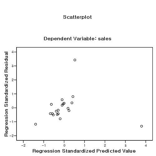
But, the result might be due to some outliers. So, check outliers by examining:

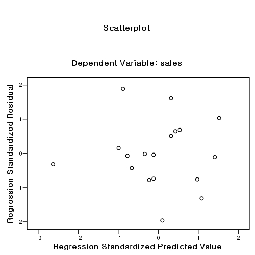
scatter plot: (z-predicted(x), z-residual(y)). The shape should be rectangular.
Mahalanobis distance score
Cook distance
Leverage

Casewise Diagnostics(a)
Case Number	Std. Residual	sales	Predicted Value	Residual
10	3.425856521	1820	867.7509889	952.2490111
a Dependent Variable: sales

두 개의 케이스를 제거한 후의 분석:
r² 값이 14%에서 70% 로 증가하였다.
독립변인 income의 b 값이 0.527406291에서 1.618765817로 증가 (따라서, t value도 증가) 하였다.

Model Summary(b)
Model	R	R Square	Adjusted R Square	Std. Error of the Estimate	Durbin-Watson
1	0.836338533	0.699462142	0.680678526	100.2063061	1.559375101
a Predictors: (Constant), income
b Dependent Variable: sales

ANOVA(b)
Model		Sum of Squares	df	Mean Square	F	Sig.
1	Regression	373916.9174	1	373916.9174	37.23788521	1.52771E-05
	Residual	160660.8604	16	10041.30378
	Total	534577.7778	17
a Predictors: (Constant), income
b Dependent Variable: sales

						Coefficients(a)
Model		Unstandardized Coefficients		Standardized Coefficients	t	Sig.
		B	Std. Error	Beta
1	(Constant)	-42.98345338	132.2567413		-0.325000094	0.749391893
	income	1.618765817	0.265272066	0.836338533	6.102285245	1.52771E-05
a Dependent Variable: sales

Normality

Normality
Data: elemapi2.sav

get file="drivename:\\elemapi2.sav".
regression
  /dependent api00
  /method=enter meals ell emer
  /save resid(apires).

examine
  variables=apires
  /plot boxplot stemleaf histogram npplot.

Homoscedasticity

Homoscedasticity
The distribution of residual along the x-values (independent values) should NOT have a pattern.

Multi-collinearity

Multicollinearity

It is about correlations among IVs
Why? . . . .

Nonlinearity

Linearity

case number

About 20 times than IV numbers.
- When you have 5 IVs, you need 5 * 20 = 100 cases.
Minimum is said to be 5 times (instead of 20 times).

Table of Contents