This is an old revision of the document!
Table of Contents
Constructing Confidence Intervals
Guessing with Confidence
The problem with precision
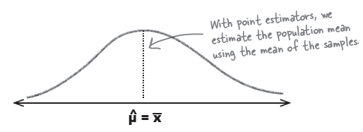
Point estimators are valuable, but they may give slight errors.
Rather than specify an exact value, we can specify two values we expect flavor duration to lie between.

The far side of each end, (a, b) is called a confidence interval.
Four steps for finding confidence intervals
Step 1: Choose your population statistic

Step 2: Find its sampling distribution

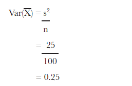
Mighty Gumball used a sample of 100 gumballs to come up with their
estimates, and they have calculated that s2 = 25. This means that

Step 3: Decide on the level of confidence
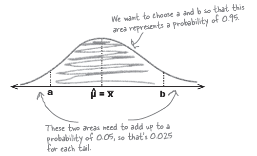
Step 4: Find the confidence limits

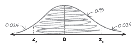
$$P(z_{a} < Z < z_{b}) = 0.95$$
$$P(Z < z_{a}) = 0.025$$
$$z_{a} = -1.96$$
$$P(Z > z_{b}) = 0.025$$
$$z_{b} = +1.96$$
\begin{eqnarray*} P\left(-1.96 < z < 1.96 \right) = 0.95 \\ P\left(-1.96 < \frac{\overline{X}-\mu}{0.5} < 1.96 \right) = 0.95 \end{eqnarray*}
\begin{eqnarray*} -1.96 < \frac{\overline{X}-\mu}{0.5} < 1.96 \\ \end{eqnarray*}
\begin{eqnarray} -1.96 & < & \frac{\overline{X}-\mu}{0.5} \nonumber \\ -1.96 * 0.5 & < & \overline{X}-\mu \nonumber \\ -0.98 + \mu & < & \overline{X} \nonumber \\ \mu & < & \overline{X} + 0.98 \\ \nonumber \\ \nonumber \\ \frac{\overline{X}-\mu}{0.5} & < & 1.96 \nonumber \\ \overline{X}-\mu & < & 1.96 * 0.5 \nonumber \\ \overline{X} & < & 0.98 + \mu \nonumber \\ \overline{X} - 0.98 & < & \mu \end{eqnarray}
(1)과 (2)에서
\begin{eqnarray*}
\;\;\; \overline{X} - 0.98 < \mu < \overline{X} + 0.98
\end{eqnarray*}
\begin{eqnarray*}
P(\overline{X} - 0.98 < \mu < \overline{X} + 0.98) = 0.95
\end{eqnarray*}
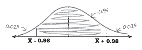
$\overline{X} = 62.7$ 이었으므로 $62.7 - 0.98$와 $62.7 + 0.98$이 구하는 공간 (interval). 즉,
$(61.72, 63.68)$
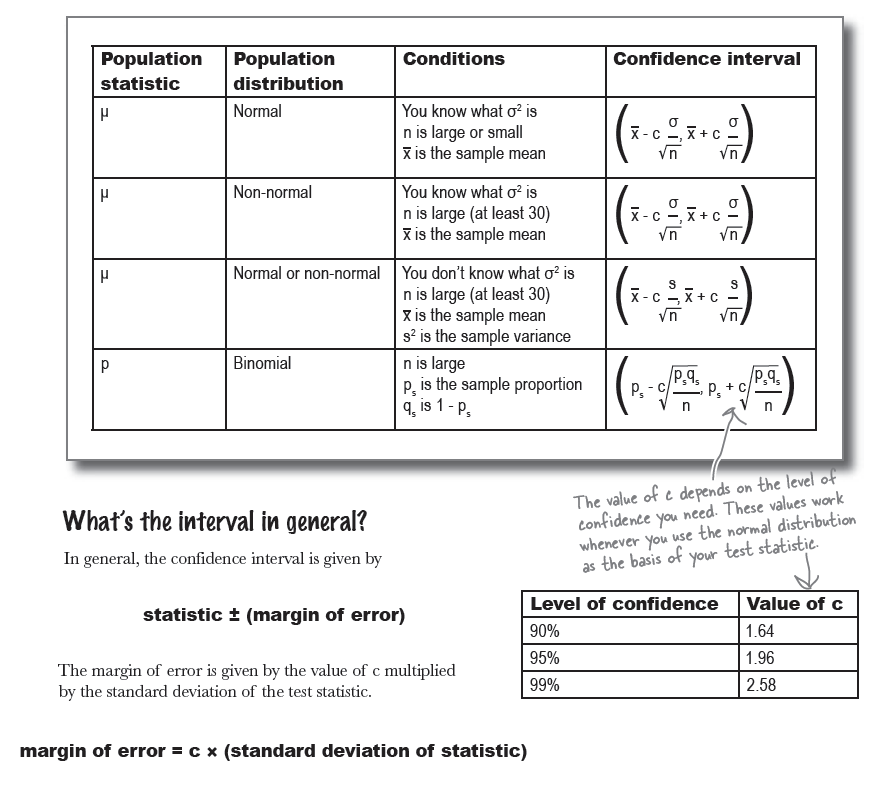
Handy shortcuts for confidence intervals
Mighty Gumball took a sample of 50 gumballs and found that in the sample, the proportion of red gumballs is 0.25. Construct a 99% confidence interval for the proportion of red gumballs in the population.
$$\left(p_{s} - c \sqrt{\frac{p_{s}*q_{s}}{n}}, \quad p_{s} + c \sqrt{\frac{p_{s}*q_{s}}{n}}\right)$$
\begin{eqnarray*} c & = & 2.58 \\ p_{s} & = & 0.25 \\ q_{s} & = & 0.75 \\ n & = & 50 \end{eqnarray*}
\begin{eqnarray*} \text{CI} & = & \left(p_{s} - c \sqrt{\frac{p_{s}*q_{s}}{n}}, \quad p_{s} + c \sqrt{\frac{p_{s}*q_{s}}{n}}\right) \\ & = & \left(0.25 - 2.58*\sqrt{\frac{0.25 * 0.75}{50}}, \quad 0.25 + 2.58*\sqrt{\frac{0.25 * 0.75}{50}} \right) \\ & = & (0.25 - 2.58 * 0.0612, \; 0.25 + 2.58 * 0.0612) \\ & = & (0.25 - 0.158, \; 0.25 + 0.158) \\ & = & (0.092, \; 0.408) \end{eqnarray*}
Just one more problem...
Step 1: Choose your population statistic
Mighty Gumball has taken a representative sample of 10 gumballs and weighed each one. In their sample, x = 0.5 oz and s2 = 0.09.
Step 2: Find its sampling distribution
The normal distribution isn't a good approximation for every situation.
When sample sizes are large, the normal distribution is ideal for finding confidence intervals. It gives accurate results, irrespective of how the population itself is distributed.
Here we have a different situation. Even though $X$ itself is distributed normally, $\overline{X}$ isn’t.
Because of small number of sample . . . .
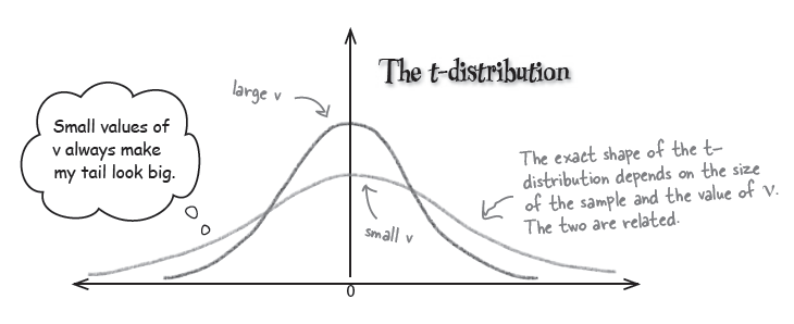
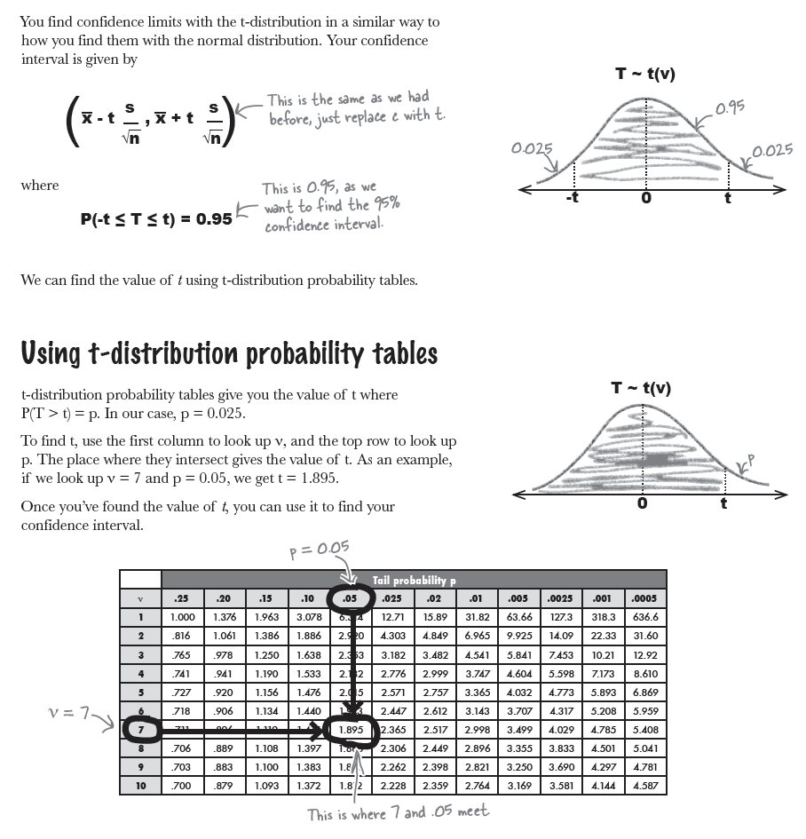
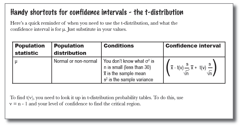
So what sort of distribution does X follow? It actually follows a t-distribution.

