Introduction

• one-way ANOVA for related, not-independent groups
• extension of the dependent t-test (one group t-test, repeated measure t-test)
• also, it is called “within-subjects ANOVA” or “ANOVA for correlated samples”
• the simplest one is one-way repeated measures ANOVA
• which requires one independent and one dependent variable
• the independent variable is categorical (either nominal or ordinal)
• the dependent variable is continuous (interval or ratio)

Test Circumstances

• one subject with repeated measures across a time period (differences of mean scores across three or more time periods)
  • participants being tested with headache drugs such as
    • group A, B, C, placebo
    • across the time periods j, k, l, m
  • testing the effect of a three-month exercise training program on blood sugar level
    • measure blood sugar level at 3 different points (pre-exercise, midway, post-exercise)
• one subject with repeated measures in different situation (treatments; differences of mean scores under three or more different conditions)
  • e.g., participant (n=30) using and evaluating three web site UI (naver, daum, and google)
  • and rate its usefulness, usability and ease of use
• data should look as follows:

Levels = related groups of the independent variable “time”

in general, the data should look

You should discern the above from normal ANOVA situation.

LOGICS

• $\text{independent ANOVA: } F = \displaystyle \frac{MS_{between}}{MS_{within}} = \frac{MS_{between}}{MS_{error}}$

• $\text{rep measures ANOVA: } F = \displaystyle \frac{MS_{between}}{MS_{within}} = \displaystyle \frac{MS_{conditions}}{MS_{error}}$

주>

• “between” 이란 단어는 독립적인 그룹 간의 비교를 의미하므로, 반복측정(repeated measure)의 경우에는 conditions라는 용어를 사용.

– Picture about here –

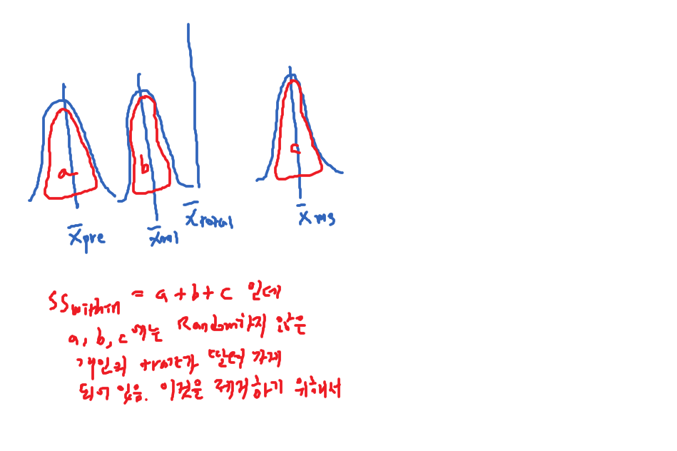
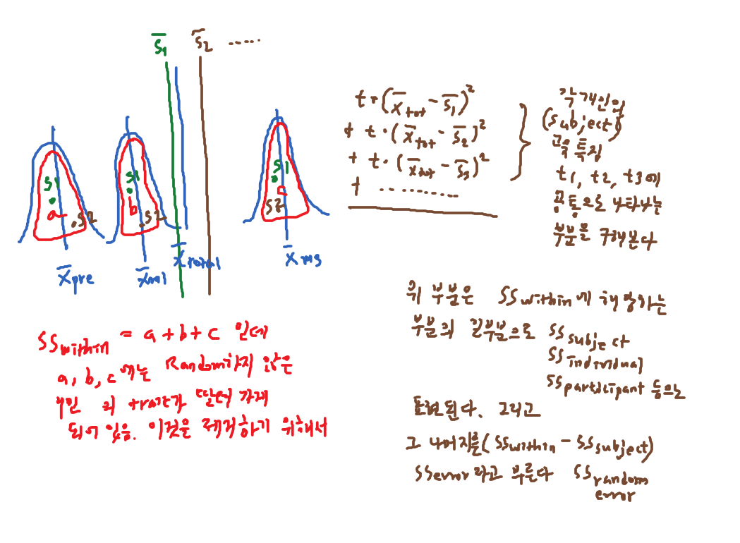
• but, $\text{SS}_\text{{within}}$ can be partitioned as
  • $\text{SS}_{\text{ subjects}}$ and $\text{SS}_{\text{ error}}$
  • that is, some of the “within variation” are carried along in each individual.
  • Among the two, we can exclude the first from SS_within
  • and solely use the latter as SS_error
  • This is to say:
    • in $\text{independent ANOVA: } \text{SS}_\text{{within}} = \text{SS}_{\text{error}} $
    • in $\text{rep measures ANOVA: } \text{SS}_\text{{within}} = \text{SS}_{\text{subjects}} + \text{SS}_{\text{error}}$
  • This means that the term SS_error will be smaller
  • But, with this SS_error, the df is going to be (n-1)(k-1)

We do this (and the below example) with an excel spreadsheet.
We also require fdistribution table to determine the null hypothesis test.

SS_total = $\Sigma{(X-\overline{X})^2} $ = 3489.2

SS_between
= SS_conditions
= SS_weeks
= $n\Sigma{(\overline{X}_{week} - \overline{X})^2}$ = 1934.5

SS_within
= $ \Sigma \Sigma{(X_{s_i.t_j} - \overline{X_{t_j}})^2}$
= $ \Sigma (411.6, 836.0, 78.0, 93.6, 135.6) $
= 1554.7

SS_participants = $w\Sigma{(\overline{X}_{participants}-\overline{X})^2}$ = 833.6

SS_residual
= SS_error
= SS_within - SS_participants
= 1554.7 - 833.6
= 721.1

OR
SS_residual =
= SS_error
= (SS_total - SS_{weeks(between)}) - SS_participants
= 721.1



df_total = N - 1 = 45 - 1 = 44

df_week = 5 - 1 = 4 = df_between

df_participants = 9 - 1 = 8 = df_subjects

df_error= (n - 1)(k - 1) = 8 * 4 = 32 = 40 - 8 = 32

df_within = N - k = 45 - 5 = 40

https://rcompanion.org/handbook/I_09.html

demo1  <- read.csv("https://stats.idre.ucla.edu/stat/data/demo1.csv")
demo1 
str(demo1) ## 모든 변인이 int이므로 (숫자) factor로 바꿔야 한다

## Convert variables to factor
demo1 <- within(demo1, {
  group <- factor(group)
  time <- factor(time)
  id <- factor(id)
}) ## 이제 pulse만 제외하고 모두 factor로 변환된 데이터

str(demo1)

demo1 data는 아래와 같다.

id	group	pulse	time
1	1	10	1
1	1	10	2
1	1	10	3
2	1	10	1
2	1	10	2
2	1	10	3
3	1	10	1
3	1	10	2
3	1	10	3
4	1	10	1
4	1	10	2
4	1	10	3
5	2	15	1
5	2	15	2
5	2	15	3
6	2	15	1
6	2	15	2
6	2	15	3
7	2	16	1
7	2	15	2
7	2	15	3
8	2	15	1
8	2	15	2
8	2	15	3

이를 정리해보면

demo1.within.only.aov <- aov(pulse ~ time + Error(id), data = demo1)
summary(demo1.within.only.aov)

> demo1.within.only.aov <- aov(pulse ~ time + Error(id), data = demo1)
> summary(demo1.within.only.aov)

Error: id
          Df Sum Sq Mean Sq F value Pr(>F)
Residuals  7  155.3   22.18               

Error: Within
          Df Sum Sq Mean Sq F value Pr(>F)
time       2 0.0833 0.04167       1  0.393
Residuals 14 0.5833 0.04167               
> 

see repeated_measures_anova_eg.xlsx

# create data
df <- data.frame(patient=rep(1:5, each=4),
                 drug=rep(1:4, times=5),
                 response=c(30, 28, 16, 34,
                            14, 18, 10, 22,
                            24, 20, 18, 30,
                            38, 34, 20, 44,
                            26, 28, 14, 30))

# view data
df

# within sujbect anova
within.aov.mod <- aov(response~drug+Error(patient), data=df)

> #create data
> df <- data.frame(patient=rep(1:5, each=4),
+                  drug=rep(1:4, times=5),
+                  response=c(30, 28, 16, 34,
+                             14, 18, 10, 22,
+                             24, 20, 18, 30,
+                             38, 34, 20, 44,
+                             26, 28, 14, 30))
> 
> #view data
> df
   patient drug response
1        1    1       30
2        1    2       28
3        1    3       16
4        1    4       34
5        2    1       14
6        2    2       18
7        2    3       10
8        2    4       22
9        3    1       24
10       3    2       20
11       3    3       18
12       3    4       30
13       4    1       38
14       4    2       34
15       4    3       20
16       4    4       44
17       5    1       26
18       5    2       28
19       5    3       14
20       5    4       30
> 
> #within sujbect anova
> within.aov.mod <- aov(response~drug+Error(patient), data=df)
> 
> 
> summary(within.aov.mod)

Error: patient
          Df Sum Sq Mean Sq F value Pr(>F)
Residuals  1   67.6    67.6               

Error: Within
          Df Sum Sq Mean Sq F value Pr(>F)
drug       1   11.6   11.56   0.139  0.714
Residuals 17 1412.6   83.10 

The above is WRONG.

within.aov.mod <- aov(response~factor(drug)+Error(factor(patient)), data=df)

summary(within.aov.mod)

> within.aov.mod <- aov(response~factor(drug)+Error(factor(patient)), data=df)
> 
> 
> summary(within.aov.mod)

Error: factor(patient)
          Df Sum Sq Mean Sq F value Pr(>F)
Residuals  4  680.8   170.2               

Error: Within
             Df Sum Sq Mean Sq F value   Pr(>F)    
factor(drug)  3  698.2   232.7   24.76 1.99e-05 ***
Residuals    12  112.8     9.4                     
---
Signif. codes:  
0 ‘***’ 0.001 ‘**’ 0.01 ‘*’ 0.05 ‘.’ 0.1 ‘ ’ 1
> 

demo1  <- read.csv("https://stats.idre.ucla.edu/stat/data/demo1.csv")
demo1 
str(demo1) ## 모든 변인이 int이므로 (숫자) factor로 바꿔야 한다

## Convert variables to factor
demo1 <- within(demo1, {
  group <- factor(group)
  time <- factor(time)
  id <- factor(id)
}) ## 이제 pulse만 제외하고 모두 factor로 변환된 데이터

str(demo1)

par(cex = .6)

with(demo1, interaction.plot(time, group, pulse,
  ylim = c(5, 20), lty= c(1, 12), lwd = 3,
  ylab = "mean of pulse", xlab = "time", trace.label = "group"))

demo1.aov <- aov(pulse ~ group * time + Error(id), data = demo1)
summary(demo1.aov)

> summary(demo1.aov)

Error: id
          Df Sum Sq Mean Sq F value  Pr(>F)    
group      1 155.04  155.04    3721 1.3e-09 ***
Residuals  6   0.25    0.04                    
---
Signif. codes:  0 ‘***’ 0.001 ‘**’ 0.01 ‘*’ 0.05 ‘.’ 0.1 ‘ ’ 1

Error: Within
           Df Sum Sq Mean Sq F value Pr(>F)
time        2 0.0833 0.04167       1  0.397
group:time  2 0.0833 0.04167       1  0.397
Residuals  12 0.5000 0.04167               

demo2 <- read.csv("https://stats.idre.ucla.edu/stat/data/demo2.csv")
## Convert variables to factor
demo2 <- within(demo2, {
    group <- factor(group)
    time <- factor(time)
    id <- factor(id)
})
demo2

with(demo2, interaction.plot(time, group, pulse,
 ylim = c(10, 40), lty = c(1, 12), lwd = 3,
 ylab = "mean of pulse", xlab = "time", trace.label = "group"))

demo2.aov <- aov(pulse ~ group * time + Error(id), data = demo2)
summary(demo2.aov)

> demo2 <- read.csv("https://stats.idre.ucla.edu/stat/data/demo2.csv")
> ## Convert variables to factor
> demo2 <- within(demo2, {
+     group <- factor(group)
+     time <- factor(time)
+     id <- factor(id)
+ })

> demo2
   id group pulse time
1   1     1    14    1
2   1     1    19    2
3   1     1    29    3
4   2     1    15    1
5   2     1    25    2
6   2     1    26    3
7   3     1    16    1
8   3     1    16    2
9   3     1    31    3
10  4     1    12    1
11  4     1    24    2
12  4     1    32    3
13  5     2    10    1
14  5     2    21    2
15  5     2    24    3
16  6     2    17    1
17  6     2    26    2
18  6     2    35    3
19  7     2    19    1
20  7     2    22    2
21  7     2    32    3
22  8     2    15    1
23  8     2    23    2
24  8     2    34    3
> 
> with(demo2, interaction.plot(time, group, pulse,
+  ylim = c(10, 40), lty = c(1, 12), lwd = 3,
+  ylab = "mean of pulse", xlab = "time", trace.label = "group"))
> 
> demo2.aov <- aov(pulse ~ group * time + Error(id), data = demo2)
> summary(demo2.aov)

Error: id
          Df Sum Sq Mean Sq F value Pr(>F)
group      1  15.04   15.04   0.836  0.396
Residuals  6 107.92   17.99               

Error: Within
           Df Sum Sq Mean Sq F value   Pr(>F)    
time        2  978.2   489.1  53.684 1.03e-06 ***
group:time  2    1.1     0.5   0.059    0.943    
Residuals  12  109.3     9.1                     
---
Signif. codes:  0 ‘***’ 0.001 ‘**’ 0.01 ‘*’ 0.05 ‘.’ 0.1 ‘ ’ 1
> 

demo3 <- read.csv("https://stats.idre.ucla.edu/stat/data/demo3.csv")
## Convert variables to factor
demo3 <- within(demo3, {
  group <- factor(group)
  time <- factor(time)
  id <- factor(id)
})

with(demo3, interaction.plot(time, group, pulse,
  ylim = c(10, 60), lty = c(1, 12), lwd = 3,
  ylab = "mean of pulse", xlab = "time", trace.label = "group"))

demo3.aov <- aov(pulse ~ group * time + Error(id), data = demo3)
summary(demo3.aov)

> demo3 <- read.csv("https://stats.idre.ucla.edu/stat/data/demo3.csv")
> ## Convert variables to factor
> demo3 <- within(demo3, {
+     group <- factor(group)
+     time <- factor(time)
+     id <- factor(id)
+ })
> 
> with(demo3, interaction.plot(time, group, pulse,
+  ylim = c(10, 60), lty = c(1, 12), lwd = 3,
+  ylab = "mean of pulse", xlab = "time", trace.label = "group"))
> 
> demo3.aov <- aov(pulse ~ group * time + Error(id), data = demo3)
> summary(demo3.aov)

Error: id
          Df Sum Sq Mean Sq F value  Pr(>F)    
group      1 2035.0  2035.0   343.1 1.6e-06 ***
Residuals  6   35.6     5.9                    
---
Signif. codes:  0 ‘***’ 0.001 ‘**’ 0.01 ‘*’ 0.05 ‘.’ 0.1 ‘ ’ 1

Error: Within
           Df Sum Sq Mean Sq F value   Pr(>F)    
time        2 2830.3  1415.2   553.8 1.52e-12 ***
group:time  2  200.3   100.2    39.2 5.47e-06 ***
Residuals  12   30.7     2.6                     
---
Signif. codes:  0 ‘***’ 0.001 ‘**’ 0.01 ‘*’ 0.05 ‘.’ 0.1 ‘ ’ 1
> 
> 

• Repeated measures one-way ANOVA by Akkelin
  • ezdata: SPSS Data file
• http://www.psych.utoronto.ca/courses/c1/chap14/chap14.html
• https://statistics.laerd.com/statistical-guides/repeated-measures-anova-statistical-guide.php

• http://rcompanion.org/handbook/I_09.html : This is an excellent example, but, difficult to swallow.